I made another math post with only differentiating the square function and integrating the identity function like in integrating zdz on the complex plane. This post is much shorter, only 7 images long and one appendix so all in all 8 images. One of the reasons I decided to write another post on this relative simple stuff is that historically speaking the square was the thing that gave the complex plane. And for some reason professional math people are completely fixated on that when they try for example find 3D complex numbers: It has to be based on some stuff with a square. Just like say the 4D quaternions from Hamilton: Basically it’s all based on the squares of the three imaginary components and an extra rule for multiplying different imaginary units.
Without much ado let me hang in the 8 images:
It is no secret that inside the profession of math at the universities they can only perform integration with a primitive when it comes to the real line and the complex plane. In the last two posts I showed you again and again how to do this on other spaces. Will the professional community ever change ways and include more spaces where you can perform integration ‘Just like on the real line’? No, after all these are university people and as such it is mostly a giant balloon of hot ego air and not much substance when it comes to math.
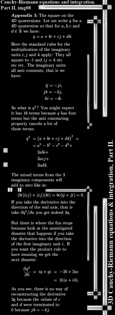
By accident I came across a work of professor Tom who happily informs his audience of the miracles of the 4D quaternions. You know for me math is a hobby, it’s an important hobby but it’s just a hobby. And because after all the subject is math I take it seriously. But decade in decade out the only thing professional math professors do is fuck around and that’s it. Here’s the link to the garbage from professor Tom: Stop 3: Multi-dimensional World These people just never make any kind of progress, if it’s the year 1990 or the present 2026 it just does not matter. They can’t go beyond the square and also they are very unwilling to go beyond the square. Let me leave my little rant with that, here’s what missing in literally all texts on quaternions: The square of a quaternion…
Ok that was it for this latest post. Likely the next post is one on magnetism in particular electron pairs in chiral molecules. Thanks for your attention.
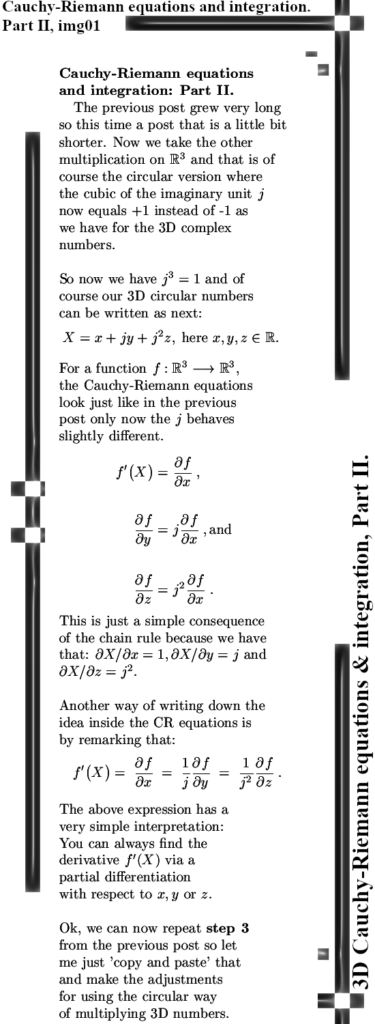
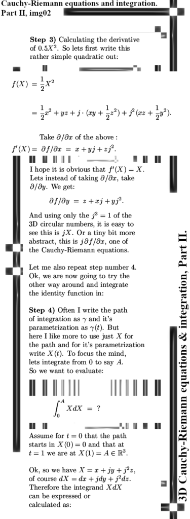
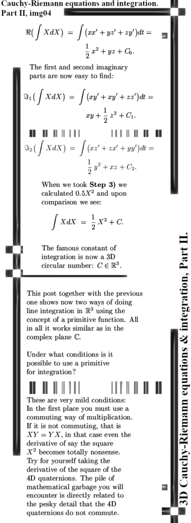
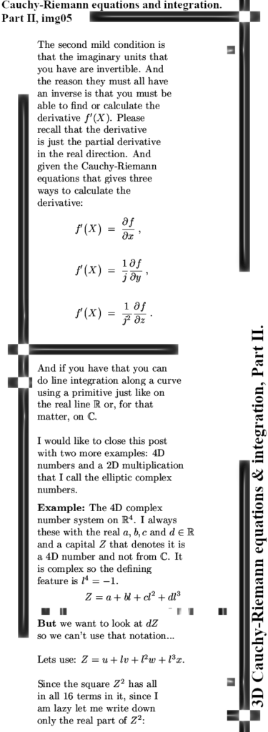
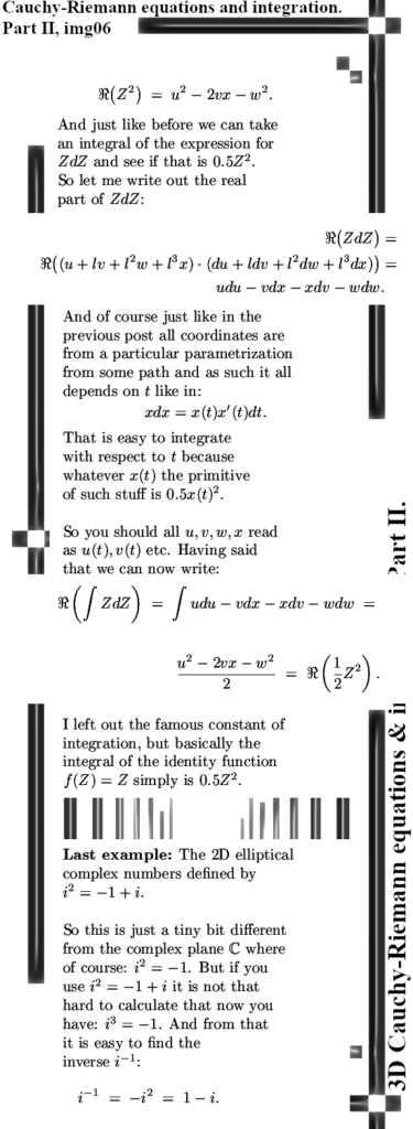
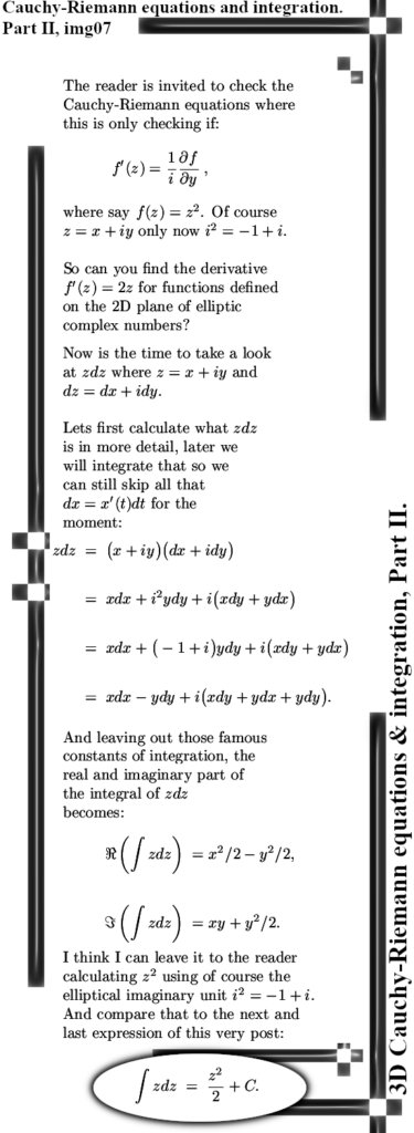
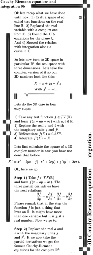
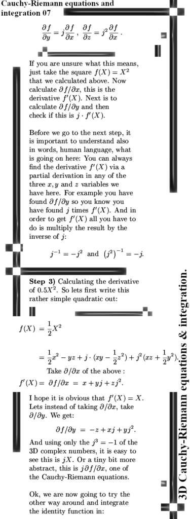
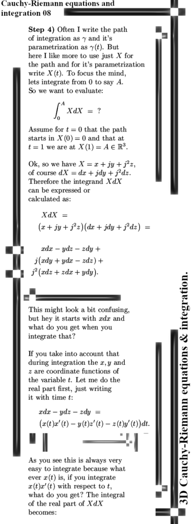
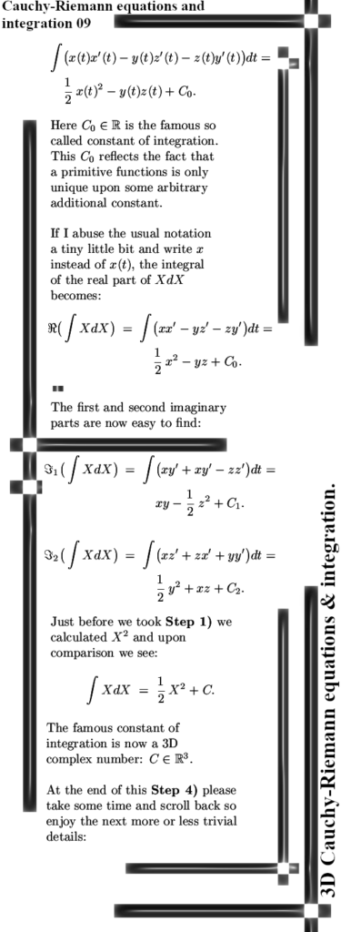
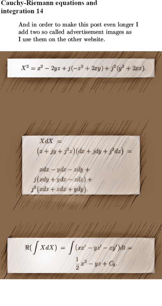
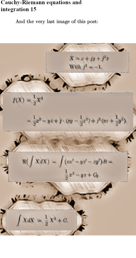
This post is about the CR equations for the 3D complex numbers, as an example we look at the next simple function there is after linear functions: the square. On us will fall the noble task of differentiation 0.5X^2 on the 3D complex numbers and of course we will find the identity function. To top it all off, after that we integrate the identity function with respect to X, so we evaluate XdX and miracle miracle we get 0.5X^2.
So more basic as this is not possible, only boring stuff like how to add two 3D complex numbers is even more basic. And for me it was actually fun to write it down one more time after so many years. Also as far as I remember, I never had differentiation and integration in one post combined. Mostly I treated them separately.
Because this subject was so elementary I allowed myself for one time to not skip a lot of stuff. Just pen down whatever crossed my mind. As a result this post is now 15 images long and I guess that is a decade long record at least.
I also included a link to a wiki about line integration in say 3D in order to demonstrate it clearly that the entire math community still can’t do a line integration in 3D using the good old concept of a primitive. Just like we integrate on the real line and the complex plane. After a third of a century of time, those people still have no clue at all. If I remember it all correctly, it is so long ago, it was in 1991 or may be 1992 I found these results. But the local professors here at the university of Groningen did not want to look at stuff like this. That’s how they do science over here…
Anyway the math part is 13 images long and I included two so called advertisement images as I use them on the other website. Ok lets now turn to the 15 images:
There was a typo in the image, now 02 May it’s repaired.
That was it more or less for this post. The previous post about circular photons and magnetic domains was a number one search result on Google within 24 hours! Now you must not think I am looking at my search ratings all the time, actually I almost never do that may be less as once a year I don’t know. But I had sought only once on “Circular light and magnetic domains” that just one day after the publishing of the last post I decided to take a look again. And to my surprise my own post on it was the no one result. And ok ok, my search text was more or less precisely the title of my post but on number one in about 20 hours of time?
You also must not jump to the conclusion that a most on the magnetic properties of an electron so fast at number one will make a dent in the attitude of the physics people at universities. My estimation is that they will keep on pretending that electrons are more or less tiny magnets. And just entertaining the idea that magnetic properties and electric properties of electrons are the same so monopole and permanent is just bad for their career. Just as the math profs do with say this post for the last 35 years. Never forget you are dealing with university people and that means most of the time it is more ego and not much science…
With that it is time to end this post and may I thank you for your attention to the matter of line integration in 3D complex space using a primitive?
I wasted a few weeks of time by making the wrong searches, I just looked for stuff related to so called Kerr microscopes and all I found every time was that the polarization of the reflected light was rotated. So that was always about linear polarization because it makes not much sense to ‘rotate’ light that is circular polarized. Ok there are of course also all kinds of elliptic polarized photons and there it might make some sense to talk about rotation of polarization but in fact those Kerr microscopes all work (as far as I know) all with linear polarization. And there is nothing wrong with that, I mean it is not forbidden or so but I wanted to see how the visibility of magnetic domains is using circular polarized light. And when I finally searched for that (visibility of magnetic domains using circular polarized light) within a minute or five I got what I wanted.
Let me very short describe what I expected and how I think it all works: 1) Electrons are magnetic monopoles and as such there are two kinds of them. 2) The photons produced by these two types of electrons have their magnetic field phase shifted by 180 degrees. 3) The way these photons react on other electrons depends on what kind of electron it is. Therefore you should see a difference for neighboring magnetic domains in a material that has magnetic domains. Furthermore the magnetic domains have surpluses of one kind of electrons and a deficit of the other kind of electrons. So that’s 4) Domains have surpluses of one kind. And, also very important, the domain walls keep these surpluses/deficits as they are. So if a domain has a surplus of say north pole like like electrons or n-electrons as I name them in the post below, the n-electrons get repelled by the domain wall.
So what are we going to see if we shine a circular light source on a piece of condensed matter that has magnetic domains (I think the authors used a film or a flat kind of material)? I will link my source file below but first we take a look at the four pictures that make up this new post:
As you see the results are very similar but also very different. If you use a standard setup for a Kerr microscope with linear polarized light and also use a so called analyser, that jacks up the contrast. And with using circular polarized light you get a much more subtle picture. What I found very interesting is that the domain walls become darker so that more or less confirms domain walls repel unpaired electrons.
This is the guy that back in the year 2000 together with David DiVincenzo formulated some criteria for qubits for quantum computing. These criteria are, as far as I know, not specific to qubits based on electron spin, but all electron spin qubit people know these criteria. Daniel is strongly interested in qubits based on electron spin, for David I do not know. What I find interesting is that how can you work for half a century on electron spin and never realize there is something wrong with the official version of bipolar magnetism that has to serve as the spin of the electron or as I often say it: It’s magnetic properties. All this garbage like anti-aligned spins in electron pairs or, also very crazy, in chemistry a non-bonding pair like in molecular oxygen has it’s electron spins aligned. All these garbage ‘results’ are only there if you view electrons as tiny bipolar magnets. If on the other hand you simply say: The magnetic properties on an electron are the same as the electric properties in the sense that is it permanent and monopole.
I want to remark that these two people are not selected because of their individual properties like belief in bipolar magnetism, but I let them stand for the entire quantum computing crowd out there. The weirdo’s that think you can explain the result of the famous Stern-Gerlach experiment via electrons that by chance either align their closed magnetic field or anti-align themselves. No my dear crowd: Bipolar magnets large and small do not anti-align themselves because that is a spontaneous rise in potential energy. And nature does not do that; there is a long long list of energy problems related to bipolar electron magnetism buy hey: Try to explain that to the quantum computing crowd in general and those working on qubits based on electron spin in particular.
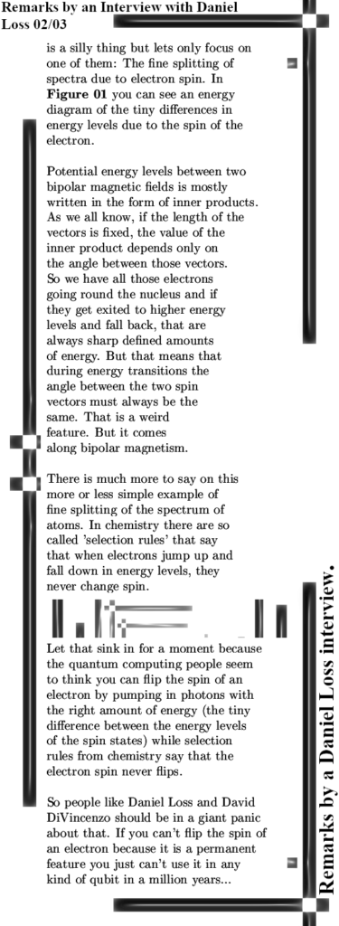
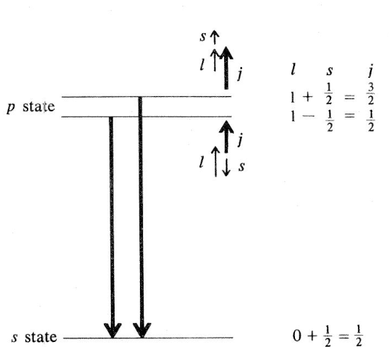
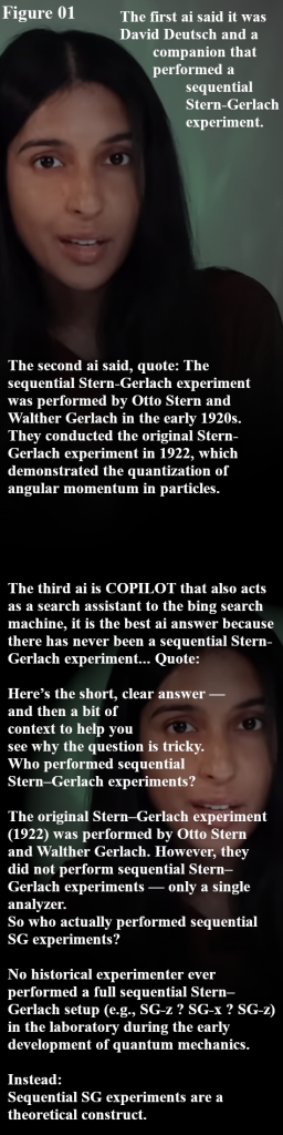
The video itself contains no new information, anyway not for me. The interviewer is as so often a person from outside physics and as such he has no clue what the quantum computing crowd means with concepts like entanglement. The video is about half an hour long, it is more a social snapshot of how it goes into the world of quantum computing and contains almost nothing worthwhile knowing. So don’t blame me if you think you are wasting your time watching it. There are three intro pictures and of course I also have one of those very famous Figure 1 images included. That makes my hobby work look very professional: Oh he has a Figure 1 in it, wow that really must be something!
Here’s the famous Figure 1 of this post: It is about the fine splitting en atomic spectra due to the monopole magnetic permanent charge each and every electron has. If electron spin was a vector as the quantum crowd always claim, how come these spectral lines are that sharp?
And finally the video itself:
That was it for this post, thanks for your attention and may be meet you again in a future post.
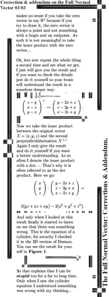
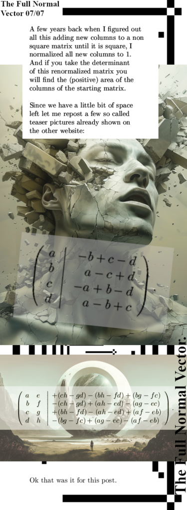
Some time back I was looking at a few recently published posts and I started scribbling a few calculations. And all of a sudden I realized something has gone wrong. Now that full normal vector does what it was supposed to do: Always return a normal vector even if there is only one minor matrix that is not singular. But sometimes you get a zero vector and that is not what you want of course. You can always work around it if it happens to you, so it is not a serous fault or so. But it’s all a tiny bit less perfect as I thought.
That full normal vector is something you can use if you want to make a non square matrix into a square one. In doing so you must craft new columns perpendicular to all previous columns and normalize them. And there is the problem of course: If you get a zero vector, you cannot normalize it to length one.
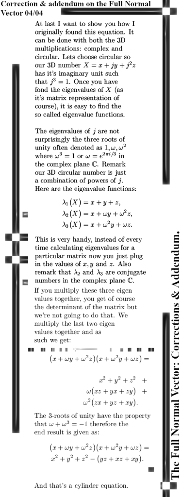
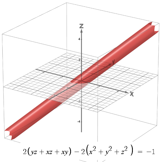
The reason I decided to write this post is that during my scribbling I soon got one of those cylinder equations that don’t look at all like the equation of a cylinder. But in the 3D numbers, both complex and circular, you can factorize the determinant with a plane and a cylinder equation. So in that sense it is very vaguely related to the 3D numbers. For 3D numbers you can factorize the determinant using it’s eigenvalues and stuff like that I always name “Eigenvalue functions” because you just plug in the coordinates of a number and voila: There are your eigenvalues. It’s much easier compared to every time by hand calculating the 3 eigenvalues every 3D number has.
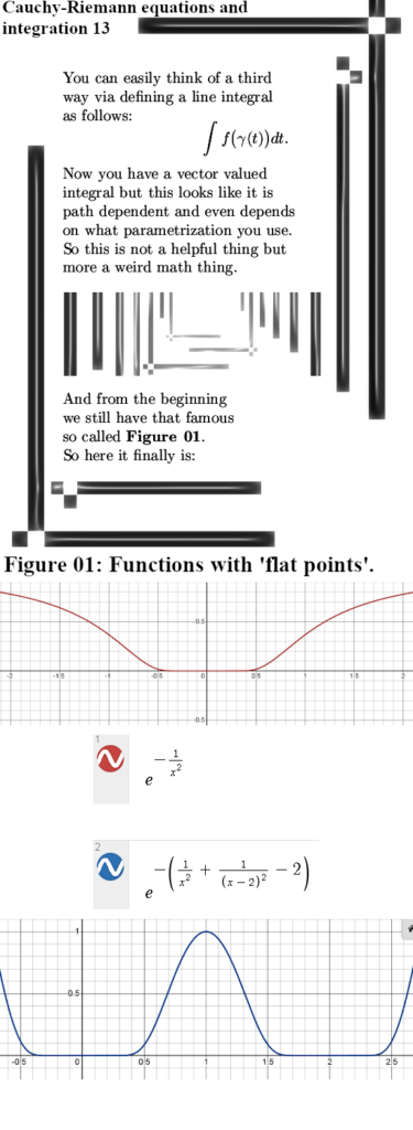
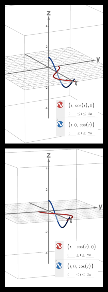
This post is four images long and an extra graph in a so called “Figure 01“. With the 3D version of Desmos, a free browser based app for drawing graphs, you can try a bit for yourself. I used two versions of the cylinder equation, don’t get confused by that because the one is only the minus of the other. That’s why in Desmos you sometimes must equal the cylinder equation to a positive number or a negative number. Here we go:
Again: If you try it in Desmos you must either use positive or negative numbers for your cylinder equation.
In case you want to know a bit more about the eigenvalue functions, just use the search function of this website and you will find plenty of stuff to think about. Ok, I hope you learned something and if not lets hope you are not one hundred % bored because math is just a boring thing or not? The next post is likely about magnetism but it is also tempting to write one more post on all the possible factorizations you can do with the determinant of 3D numbers and the many ways there are to find the 3D complex exponential as the intersection of a whole lot of geometrical objects. We’ll see.
A few years back Nobel prizes were rewarded for all that ‘faster than light’ stuff related to entangled particles (or photons) and the weird belief that particles far apart can more or less instantly communicate with each other.
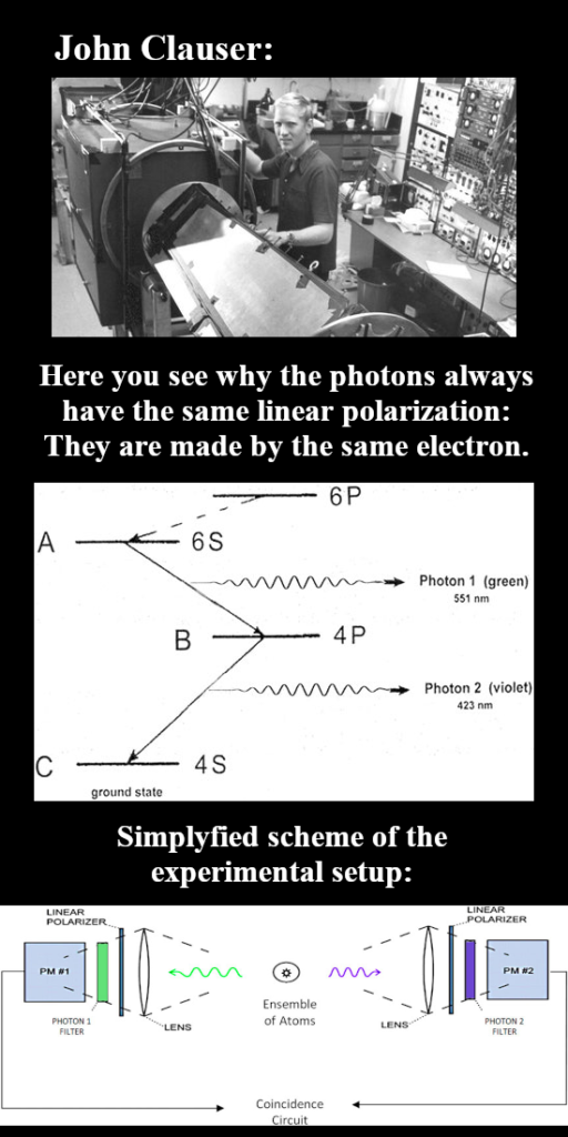
Last year 2025 (by the way happy new year) we looked in details to the first experiment from John Clauser who used cascading electrons to generate pairs of photons and he got the Nobel prize because he showed that those photons always have the same linear polarization.
Since the year 2015 I started seriously doubting that electrons are indeed tiny bipolar magnets as a possibility to explain the results from the Stern-Gerlach experiment from the year 1922. Back in the time when people tried to explain this result of Otto Stern and Walter Gerlach in the letters they did send to each other it often started with the Gauss law for magnetism and that they ‘should find a solution within this framework of the Gauss law’.
So it never dawned on them that instead of finding a solution within this Gauss framework (magnetic monopoles do not exist) their scientific task should have been: Checking if the Gauss law for magnetism is indeed valid for unpaired electrons. After all, electrons being magnetic monopoles is indeed a perfect explanation for the Stern-Gerlach experiment. But no they did not do it, no one dared to take on the Gauss law that after all is just a fancy piece of math not rooted in any experimental evidence.
That is why even today in this new year 2026 we have crazy stuff like electrons that anti-align themselves with an applied external magnetic field like they did in the SG experiment explanation. And the most crazy thing in my view is the official version of the electron pair where the present day belief is still that because of the Pauli exclusion principle the electrons must have different spin numbers while in practice this simply means the two tiny magnets somehow must be anti-aligned to form a pair while from chemistry we know that electron pairs are very important in keeping molecules together.
But let me stop ranting against the belief that magnetic monopoles do not exist and turn to the beef of why I selected this video: It is all that Bell theorem stuff that says or validates all those ‘faster than light’ kind of collapsing of the wave function that they think actually happens. There is an old proof out that proves that Einstein’s idea’s of so called hidden variables cannot be true. It was only last year in 2025 that I looked into that and guess what? This proof uses the results of a repeated or sequential Stern-Gerlach experiment that gives all those probabilities for measuring electron spin. There is only one little pesky detail: In a century of time there has never ever such an experiment done. And if my idea’s of simply electrons having a permanent magnetic charge, just like their electric charge, are true, in that case measuring electron spin is the same as measuring the electric charge of the electron: It will always be the same no matter what. So that is why John Clauser always had the same linear polarization in his pairs of photons, the root cause or the ‘hidden variable’ if you want to frame it that way of finding always equal linear polarity is that the photons are made by the same electron. You really don’t need all this ‘faster as light’ crazy stuff to explain the outcome of the experiment John Clauser did.
I am more or less planning to look in this new year a bit deeper into all those other experiments done that show the ‘faster than light’ weirdo stuff but almost all experiments use crystals that do the parametric down conversing thing and break down one photon into two lower photons with opposite linear polarization. In my view the only logical explanation using electron permanent monopole properties is that an electron pair gets ejected into a higher energy state and later falls down and as such it will always generate an electron pair with opposite linear polarization.
But lets turn to the video: If electron spin is just a permanent monopole magnetic charge, in that case measuring electron spin is not probabilistic at all and as such the ‘proof’ as presented in the video is clear cut wrong. You can find the video at the end, this post is 3 images and one extra so called Figure 1. Here we go:
Furthermore if electron spin is a permanent monopole feature and depending on the kind of magnetic charge is what gives the two opposite polarization states of the photons they produce. As such the photon pairs as mentioned in the video are never in a superposition let alone that measuring one photon’s polarization leads to a collapse of the wave function and forces the other photon to take on the opposite (linear) polarization. And as such there is no ‘faster than light’ stuff going on at all.
And finally the video:
It has to be remarked that both Mithuna Yoagnathan and Derek Muller do nothing strange here. All physics professionals believe this kind of weird stuff to the extend there are even Nobel prizes handed out for this kind of crap. So both Mithuna and Derik are nice people and do only what is accepted as truth. Even the usage of these faulty probabilities related to a sequential or repeated Stern-Gerlach experiment is what they all do while bragging that physics is the only five-sigma science… Well no it just isn’t, never ever a sequential Stern-Gerlach experiment was performed there is also zero experimental validation for their fantasy that monopoles are tiny bipolar magnets. Another very fundamental piece of experimental validation that is missing is that if it was true that electrons are tiny magnets, in that case they will not be accelerated by a constant homogeneous magnetic field. That is a cornerstone of their thinking but once more: Where is that fucking experimental validation for this?
This year a couple more video’s were published on youtube regarding this subject of the non-existence of 3D complex numbers but I skipped those and did not comment a thing. So why this video? Well those ‘proofs’ always have some things in common namely the idea that there are imaginary units in say 3D or 5D space that square to minus one. And after that those people do some calculations or math manipulations, find something that contradicts and voila the conclusion is: 3D complex numbers do not exist. Some people, but not many, are a bit sharper by stating this proofs that there is no 3D extension that includes the 2D complex plane.
But 3D or 5D or any dimension numbers do exist in there own way. In 3D space there is an imaginary unit who’s third power equals minus one, in 5D space the fifth power is minus one etc etc. And in all of those spaces you can do complex analysis because you can differentiate and perform integration ‘just like’ in the complex plane. As a comparison on those overhyped quaternions you can’t even differentiate the function that squares a quaternion. Those 4D quaternions have their own right of existence but they are not the 4D complex numbers, but I digress.
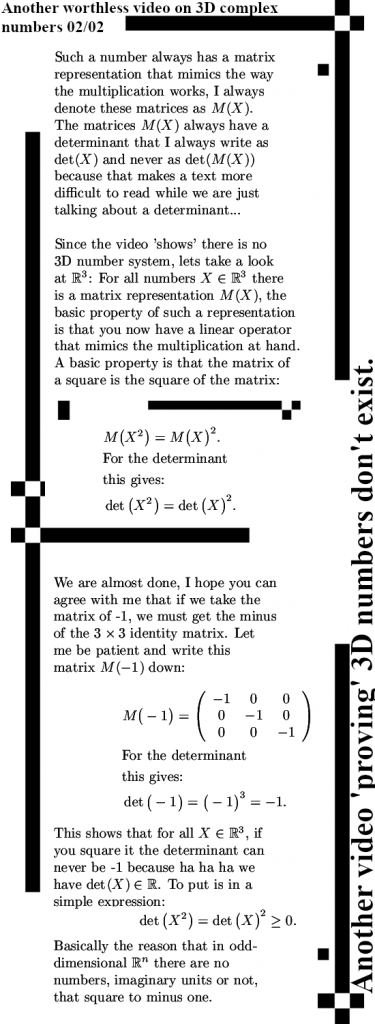
I wrote a very small math post, it is only two images long, with a proof as simple as possible that shows in real spaces with an odd number for the dimension, there are no numbers that square to minus one.
Now we all know that on the real line there is nothing that squares to minus one and in all other higher dimensional spaces if we take the determinant we get always get a real number. As such there is no determinant of any number that squares to minus one. And if you calculate the determinant of -1 (as a matrix in odd dimensions) you always get -1…
The proof below is all utterly simple but it’s relevance lies more into that it now goes for all multiplications in one single strike. So not only the so called complex multiplication but just everything that is a multiplication. If for some strange reason you want to think a bit of what all can pass as a multiplication, just use the search function of this website and search for big E. Big E is just a multiplication table although I present it like a square matrix for reasons that are obvious if you read that post.
At last I want to remark that although the title is a bit negative, I wish the composer of the video good luck with his math travels. That, by the way is the name of the video channel: Math Travel. Let me first post my two images and later the video.
Ok, lets now all smile and wave at youtube so the next video will get shown to you:
Well that was it my dear reader, thanks for making it all to the end with all that boring math stuff and so.
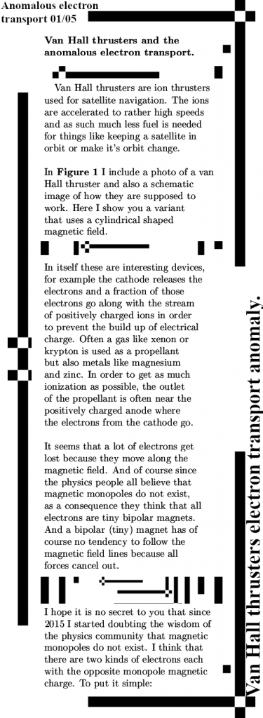
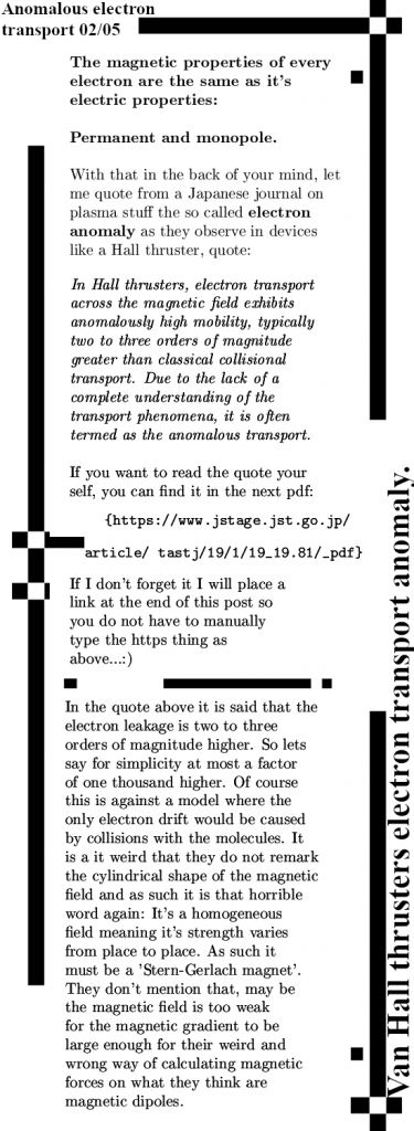
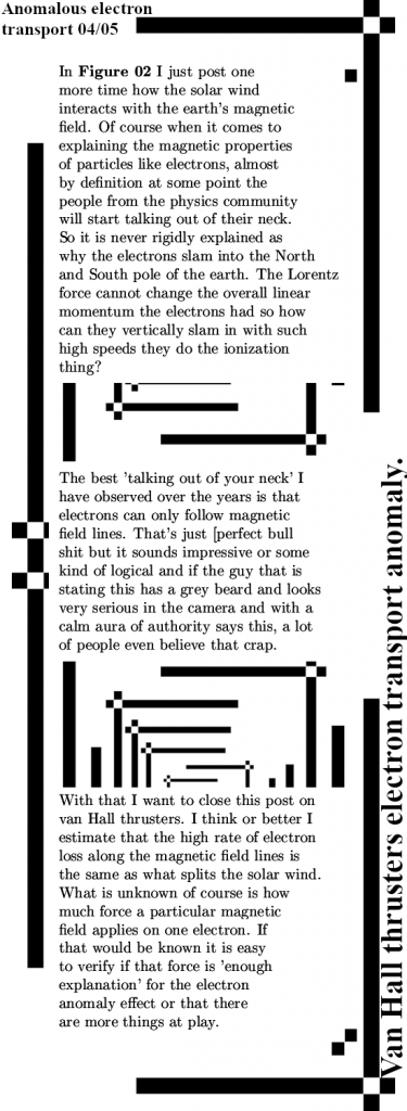
If you have never looked at these kind of devices, if you want to understand the problem of the anomalous electron transport you can look in figure 01 below. Or look it up on the internet, van Hall thrusters are at present day a common tool or device in satellites. These ion thrusters need much less propellant compared to chemical thrusters for keeping the satellites in their orbit. This post is based on an article on some Japanese website on these kind of space devices. It seems that there is much more electron loss along magnetic field lines as their collision models predict. According to their publication it is up to three orders of magnitude higher as their expectation, that is up to a 1000 times too much. And although their article never says it explicit: of course they make use of the electron as a tiny dipole magnet and as such it is neutral to magnetism. In my understanding of reality that is crazy as hell, why should an electron have only one magnetic charge and two magnetic poles? But electrons being tiny magnets is a deep held belief inside the physics community and that is why observe so many totally crazy explanations when the magnetic properties are a part of the explanation of some set of observed properties.
For example in the case of the explanation of the Stern-Gerlach experiment it is the anti-alignment of the electrons with the magnetic field that explains the split in two beams. And of course when explaining the SG experiment they often tell you about the fundamental probabilistic nature of measuring electron spin and therefore the probabilities of a neutral silver atom going up or down is 50%. We are the 5-sigma science, nothing beats us!
But if the same people have to explain the Einstein-de Haas effect, that is also something with electron spin and a vertical magnetic field, now the explanation is always that all electrons align their bipolar spin because they feel a torque because of the applied magnetic field. So now the logic is all electrons do the same while in the SG experiment it is the fundamental probabilistic nature that explains the experimental results.
If you use the not so hard to understand idea that the electric and magnetic properties of the electron are the same, as such electrons are permanent magnetic monopoles just as they are electric monopoles, if you use that idea stuff like electron pairs make much more sense: They pair up because they have opposite magnetic charges and that’s why the electron pair is neutral under (weak) magnetic fields.
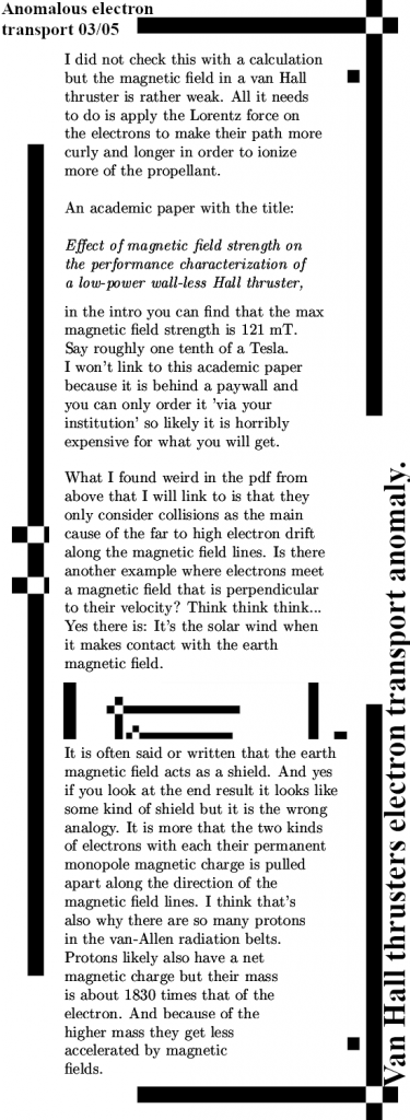
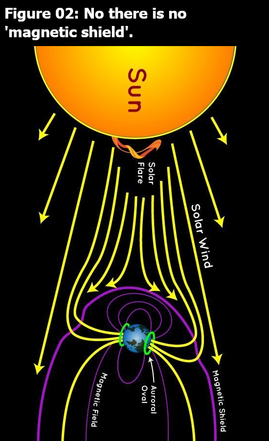
As a funny side note, if you look at the official explanation for the above two mentioned experiments, those explanations are always a combination of things that sound or look logical. But over the different experiments it is always some stuff with electrons and a vertical magnetic field, so the explanations should not differ so very much (from 100% alignment because of torque to 50/50% alignment because of the fundamental probabilistic nature of measuring electron spin. If you look at it, it looks a lot like those modern Large Language Models or LLM’s work: When an LLM gives you an answer all of it is made up stuff. Some parts are true and some parts are just untrue and a whole lot of in between stuff. But the LLM’s can’t tell what part is true and what part is a bit less truthful. It just sound logical like the explanations from physics professors when they explain this or that experiment. But enough of the talk, this post is just 4 images long and there are two additional figures. If you don’t know how van Hall thrusters work, look that up in figure 01 or find something on the internet for yourself. In figure 02 I included a picture of the earth magnetic field and the solar wind because that is another down to earth simple example of how electrons move along magnetic field lines. Ok, let me hang in the pictures and I made a small error with the ‘countdown’ number, it should read 01/04 instead of 01/05 but I leave it as it is and won’t repair it:
Ok this post was more or less based on just one pdf, here it is: Pdf article:
Link used: https://www.jstage.jst.go.jp/article/tastj/19/1/19_19.81/_pdf
Ok that was it for this post, let me try to publish it via the method of hitting the ‘Publish’ button. Thanks for your attention and see you in a new post.
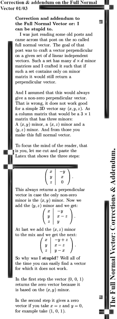
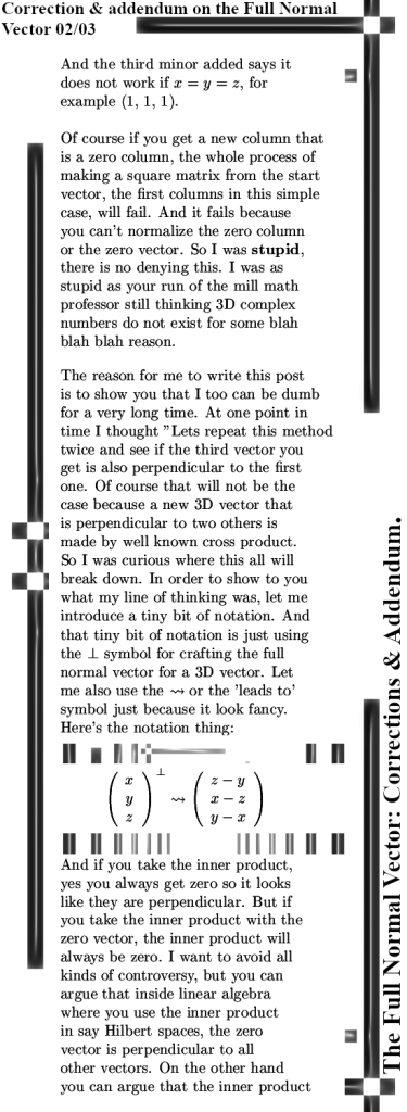
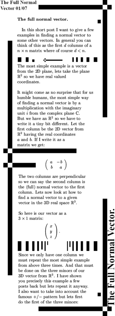
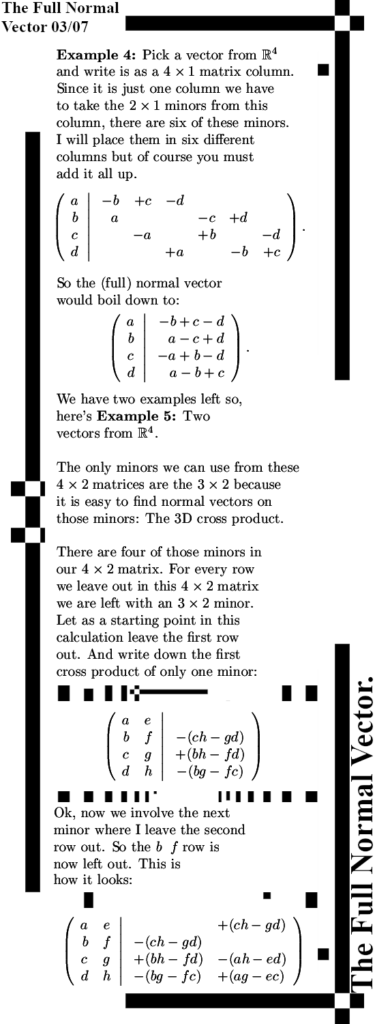
In this post we work mostly on the 4D real space only and I just show you a bunch of example as how to construct a normal vector to a given set of independent 4D vectors. So I start with just a 4D vector and construct a so called full normal vector to it. For readers who follow this website longer, yes I borrowed this title from the title of the pdf on the matrix version of the theorem of Pythagoras. That was something like the Full Theorem of Pythagoras written by Charles Frohman.
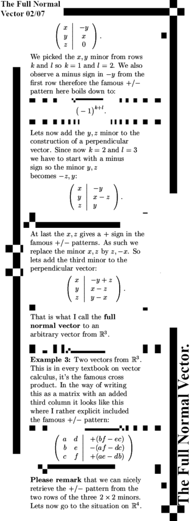
The first two examples are finding a normal vector in 2D and 3D real space and that is not very hard of course. Than the 2D and 3D results are used for all the 4D vectors of the rest of the post. Anyway the first serious example is just a 1D vector and of course in a 4D real space there is a 3D space perpendicular to each non-zero 1D vector. So it is not a unique vector in the sense like 3D where the cross product always returns a vector with a unique direction. But these full normal vectors are such that whatever the input is, it will always produce an outcome or a vector perpendicular to the given one(s).
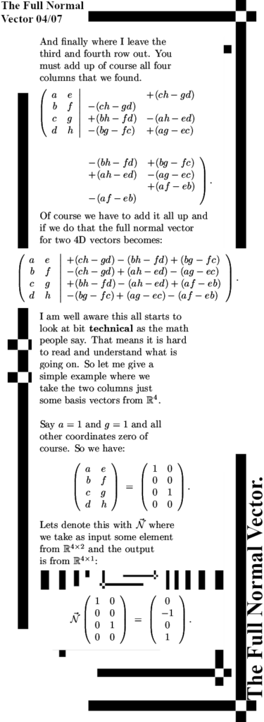
After the 1D example the next example is two 4D vectors or as I always formulate it: The first two columns of a matrix. Because we have two columns in this example we can use the good old cross product and apply that on the 4 minor 3×2 matrices there are in these two columns. That gives the full normal vector in the case of two columns.
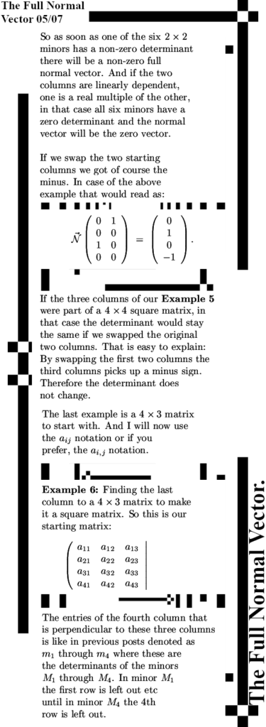
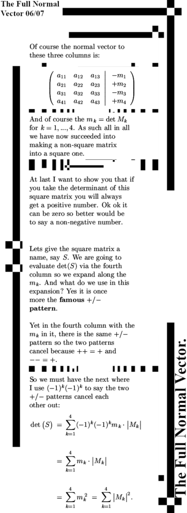
An implicit goal of this post is understanding a bit more about how determinants react on these original columns and the added extra ones. All added extra columns are perpendicular to all previous ones. So if we have that in a square matrix we can simply normalize all added extra columns to 1 and the determinant will nicely spit out the ‘volume’ of the thing we started with: A vector, a parallelogram or a 3D parallelapipid in our 4d real space.
This post is seven pictures long and if you understand all of it’s content you are now capable of always making a 4D vector into a square 4×4 matrix.
Ok, that was it for this post. In case you have never seen the Frohman pdf that all started this a few years back, here it is: The Full Pythagorean Theorem.
In the year 2022 the Nobel prize in physics went partially to John Clauser for the experimental proof or validation of quantum entanglement. This experiment was the first to probe the idea’s of John Bell and as far as I know this experiment differs from all later experiments that often use that so called “Parametric Down Conversion” stuff to get their entangled photon pairs. With the down conversion method where one photon gets smashed in two, the linear polarization of the photons is opposite to each other. So my idea was: Likely sometimes an entire electron pair gets exited and falls back. But it is very very hard to verify such a claim via experiments on the crystals that actually do this down conversion of photon energy. But the original experiment from John Clauser uses calcium atoms and a cascade of one electron going down two energy levels. And, that is important of course, here the two photons always have the same linear polarization. I am now into the 11-th year of looking at electrons as magnetic monopoles, in particular with a permanent monopole charge just like the electric charge of an electron. For years and years it looked logical that circular photons would be produced by these two kinds of electrons and the opposite magnetic charge caused the two different circular (or elliptical) photons. Only this year it dawned on me that the two different kind of linear photons have the same origin: The two different magnetic monopole charges and electron can have. It has it’s own logic, the idea of electrons as magnetic monopoles finally makes sense of say the electron pair where the Pauli exclusion principle (opposite spins) is only a bag of nonsense if you view electrons as tiny magnets or the bipolar magnetic model that is commonly believed in.
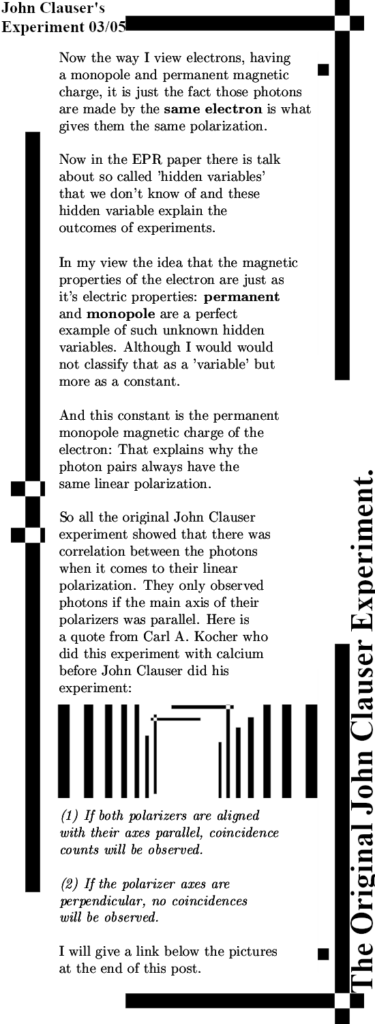
Here in the original John Clauser experiment it now has it’s own logical explanation too: John could not control what kind of electron got exited, as such he got different polarization all of the time but these polarizations for the pair of photons were always the same. A guy named Kocher did the first experiment with this calcium stuff I believe it was in the 1960-ties. He summarized the results in a beautiful manner:
(1) If both polarizers are aligned with their axes parallel, coincidence counts will be observed.
(2) If the polarizer axes are perpendicular, no coincidences will be observed.
If you want to read what Kocher wrote, at the end I have a link for you. So now we understand the root source of the experimental results from Clauser, it is also clear that this is not entaglement in the sense of a superposition of photon polarization as often portrayed as a so called Bell state. All of the time the photons had already their polarization.
It is NOT that measuring one photon makes the other have the same polarization, all of the time they already had theirs. And there is also a relative easy way to verify that the photons might be (strongly) correlated but do not influence each other: If you have access to so called entangled photons, send one of them through a quarter wave plate so it becomes an elliptic photon. Now check if the other photon is also elliptic, if I had to bet on the outcome I would say that the two photons do not influence each other.
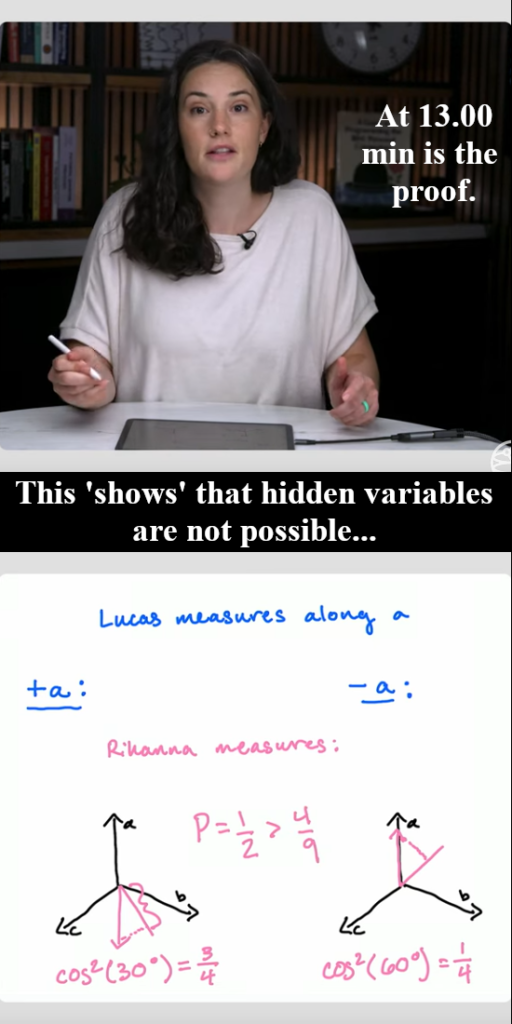
This post is five images long while I added two additional figures. And after that there is another video from Qiskit IBM quantum computing where it is ‘explained’ that hidden variables explaining the photon correlation do not exist. In figure 3 you see a screen shot of the video. And of course the link to Kocher’s summary paper.
In the next Figure 1 you see what I think are the two linear polarization states of a photon: their magnetic fields are phase shifted by 180 degrees. This introduces all kinds of subtleties that are not discussed now but for example if the electric field of a photon is vertical, you still have two kinds of photons. (Where of course the official version of linear polarization is the direction of the electric field of a photon where it’s magnetic part is always left out and not talked about.) In Figure 2 you can see John Clauser at work and a simplified energy level of calcium atoms for the cascading electron.
I left out stuff like the speed of light and the frequency of the photon.
In quantum mechanics there is also some kind of proof that the so called hidden variables do not exist. I never looked in the (historical) details of it. But the few times I observed such a ‘proof’ it is always that when measured the quantum stuff, there is always that fundamental probabilistic stuff. I think that’s wrong when it comes to say electron spin (the permanent magnetic charge) and as such the photons they produce can also never be in a superposition as say in the Bell state. It is about 13 minutes into the video where the lady does the magical “Hidden variable do not exist” kind of proof. By the way this is the same lady I showed you some weeks ago where she claimed that a repeated or sequential Stern-Gerlach experiment was done many times. But there is no successful sequential SG experiment done ever, if there was it would very very likely be in the annals of the Nobel prize and it’s just not there. A successful sequential SG experiment would not only validate the official belief in the probabilistic nature of measuring electron spin, it would also destroy all my findings into electrons being magnetic monopoles.
So my dear physics community: Bring it on what you have!
For me this is not very convincing.
And now for the video from Qiskit, IBM quantum computers:
And lets not forget the summary to a very early experiment measuring photon linear polarization using the calcium electron cascading mechanism: Quantum entanglement of optical photons: the first experiment, 1964–67 Link used: https://www.frontiersin.org/journals/quantum-science-and-technology/articles/10.3389/frqst.2024.1451239/full