Monthly Archives: October 2021

De Padé approximations; why are they so good?

Already a few years back I wanted to write a post on the so called de Padé apprximations because they are so good at taking the logarithm of a matrix. For me the access to an internet application that calculated those logs from matrix representations was a very helpful thing to speed things up. It would have taken me much much longer to find the first exponential circle on the 3D complex numbers if I could not use such applets.
But in the year 2018 pure evil struck the internet: the last applets or websites having them disappeared to never come back. Ok by that time I had perfected my method of simply using matrix diagonalization for finding such logs of matrices. You can still find it easily if you do an internet search on ‘Calculation of the 7D number tau‘.
Yet in the beginning I only had such applets as found on the internet and I soon found out that using the so called de Padé approximation always gave much better results compared to say a Taylor approximation.
It is not very hard to understand how to perform such a de Padé approximation. Much harder to understand is how de Padé found them, after all it looks like a strike of genius if this works. The genius part is of course found in the stuff you can simply neglect in such approximations, at first it baffles the mind and later you just accept it that you are more stupid as de Padé was…;)
Anyway this week I stumbled upon a cute video and as such I decided to write a small post upon this de Padé stuff. (On the shelf are still a possible new way of making an antenna based on the 3D exponential circles and some updates on magnetism.)
So let us first take a look at the video, here we go:

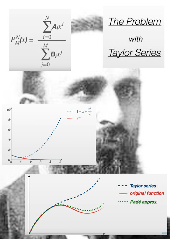
As you see the basic idea is pretty simple: you use those two polynomials to ‘approximate’ that Taylor series and as a bonus you have a much better approximation of the original function. All in all this is amazing and it makes you wonder if there are methods out there that are even better compared to this de Padé approximation.

Now you can choose beforehand what degree polynomial you use in the nominator and denominator. There are plenty of situations where this brings a big benefit like in the video they point out the divergence problems of say the sine function that is bounded between +1 and -1 on the real axis. The Taylor approximations always go completely beserk outside some interval where they fit quite well. With the appropiate choice of the degrees of the polynomials in the de Padé approximation you can avoid this kind of stuff.
In my view the maker of the video should also have pointed out that a de Padé approximation can have it’s own troubles when you divide by zero. And when the original function never has such a pole at that point, the de Padé approximation also goes very bad. These de Padé approximations
are indeed much better compared to the average Taylor approximation but they are not from heaven. You still have to use your own brain and may be that is a good thing.

De Padé still rules in the year 2021, likely it was a good idea to start with.

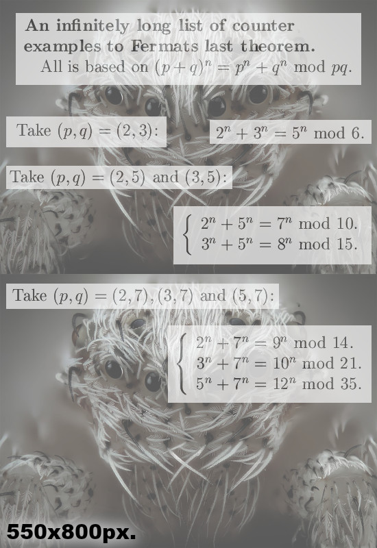
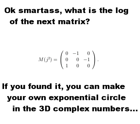
In this post I did not cover the matrices and why a de Padé approximation of the logarithm of a matrix is good or bad. If you want to find exponential circles and curves for yourself, use those applets mostly on imaginary units who’s matrix representation has a determinant of +1. In case you want to find your very first exponential circle, solve the next problem:

Ok, it is late at night so let me hit that button ‘publish website’ and see you around.

A infinite list of counter examples to the last theorem of Pierre de Fermat.

This is a very simple post, all it contains is a list of the most simple counter examples to the last theorem of Fermat. You might wonder, if it is that simple, why take the trouble and post it? Well sometimes it is important to stress the obvious and say for yourself: there is not much reaction from the math professionals so although it is utterly simple it could be that even that is once more too difficult…

These most simple counter examples are all based on two (different) prime numbers and how they behave under exponentiation while taking that modulo the product of those two prime numbers. The most simple example is given by 2^n + 3^n = 5^n mod 6. For n you can only take natural numbers because inside the ring of integers modulo 6 the two prime numbers 2 & 3 do not have an inverse and as such 2^(-1) and the likes simply do not exist. Remark such counter example via some exponential orbit are always periodic, so each and every counter example to the last theorem of Fermat only adds a finite number of ‘actual’ counter examples. In the above example the period is 2 because for n = 3 we already have 2^3 + 3^3 = 5^3 = 5 mod 6.
I organized the list in a simple manner: We like at pairs of prime numbers say (p, q) and the q is always the plafond or maximum prime allowed.
For example the plafond q = 13 yields the following pairs: (2, 13), (3, 13),
(5, 13), (7, 13) and (11, 13).
The reason for doing so is that it is now very obvious it is a one dimensional list of counter examples to the last theorem of Fermat. You can now, if you wanted it, make a one to one correspondence between the set of natural numbers and the list of counter examples.

Another reason for writing this post was that I wanted to experiment a bit with other backgrounds in the pictures used. In the list of counter examples I used two of those beautiful photo’s from the Nikon small world contest. If you have never seen them, look it up on the internet. Althugh those Nikon photo’s are very beautiful I do not think they form a good background to the math as published in the futute so I stick to my old backgrounds I just guess. I always make my math pictures with a very old graphics program that only runs on windows XP. My graphics program is so old that when I save something as a jpg format picture, the program always informs me how long it will take to send it over 28kB telephone modem… Yes, not even a 56 kB modem but a 28 kind of modem. That shows more or less how old my graphics program is but making those kind of backgrounds with say a modern version of GIMP is extremely hard and very laborsome. I like GIMP too but that old program still has features that GIMP is bad at delivering.

Another problem is the picture size under use in a WordPress website. When I started this website about six years ago I could not use any longer my favorite size of 550×1100 pixels. It did not display properly. Anyway only now six years later I dived into that problem again and it seems that WordPress makes 3 pictures of every picture you upload:
1) A thumbnail,
2) A display picture that is not ‘too large’ and
3) Your original upload visible after clicking on the display picture.

There are all kinds of issues with that; if one of my original uploads contains an error and I correct it, that never shows up on the display pictures. So I repair a fault but it does not show up. Only when I rename my faulty picture the correction of the fault is there. But that is frustrating on a lot of levels because now the natural naming of my math pictures gets distorted for no reason at all. For example if a picture has the file name 11Aug2021=Frey_elliptic_curves_are_stupid05.jpg and I have to repair a fault that is in it, I have to make the name different from the other pictures and that is weird. You can only delete your original upload and not the extra pictures that WordPress generates. In that sense it is welcome to the Hotel California where you can checkout any time you like but you can never leave.
If my expectations are correct, the first picture will display properly while the second one is likely too small but if you click on it you will see the correct version of stuff:

This displays properly…
You see, it cannot handle a picture that is 1440 pixels high…

Why my version of WordPress does not show the larger picture is unknown to me. Likely I must change some settings but I do not have a clue. Luckily it is still readable so may be this is a good time to say goodbye and until the next post and so.