To be a bit precise: I think two spaces are different if they have a different form of multiplication defined on them. Now everybody knows the conjugate, you have some complex number z = x + iy and the conjugate is given by z = x – iy. As such it is very simple to understand; real numbers stay the same under conjugation and if a complex numbers has an imaginary component, that gets flipped in the real axis.
But a long long time ago when I tried to find the conjugate for 3D complex numbers, this simple flip does not work. You only get advanced gibberish so I took a good deep look at it. And I found that the matrix representation of some complex z = x + iy number has an upper row that you can view as the conjugate. So I tried the upper row of my matrices for the 3D complex and circular numbers and voila instead of gibberish for the very first time I found what I at present day name the “Sphere-cone equation”.
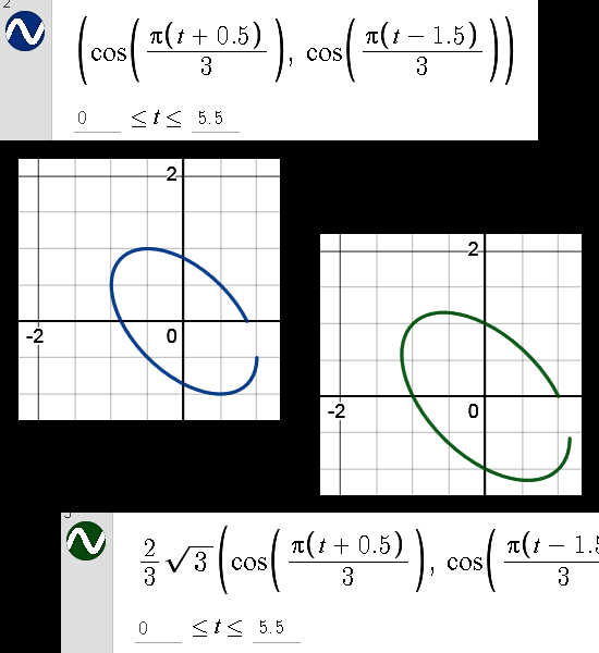
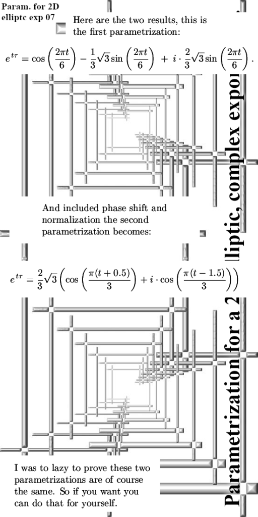
I never gave it much thought anymore because it looked like problem solved and this works forever. But a couple of months ago when I discovered those elliptic and hyperbolic versions of 2D numbers, my solution of taking the upper row does not work. It does not work in the sense it produces gibberish so once more I had to find out why I was so utterly stupid one more time. At first I wanted to explain it via exponential curves or as we have them for 2D and 3D complex numbers: a circle that is the complex exponential. And of course what you want in you have some parametrization of that circle, taking the conjugate makes stuff run back in time. Take for example e^it in the standard complex plane where the multiplication is ruled by i^2 = -1. Of course you want the conjugate of
e^it to be e^-it or time running backwards.
But after that it dawned on me there is a more simple explanation that at the same time covers the explanation with complex exponentials (or exponential circles as I name them in low dimensions n = 2, 3). And that more simple thing is that taking the conjugate of any imaginary unit always gives you the inverse of that imaginary unit.
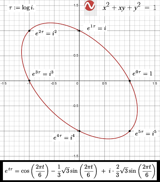
And finding the inverse of imaginary units in low dimensions like 2D or 3D complex numbers is very simple. An important reason as why I look into those elliptic complex 2D numbers lately is the cute fact that if you use the multiplication rule i^2 = -1 + i, in that case the third power is minus one: i^3 = -1. And you do not have to be a genius to find out that the inverse of this imaginary unit i is given by -i^2 .
If you use the idea of the conjugate is the inverse of imaginary units on those elliptic and hyperbolic version of the complex plane, if you multiply z against it’s conjugate you always get the determinant of the matrix representation.
For me this is a small but significant win over the professional math professors who like a broken vinyl record keep on barking out: “The norm of the product is the product of the norms”. Well no no overpaid weirdo’s, it’s always determinants. And because the determinant on the oridinary complex plane is given as x^2 + y^2, that is why the math professors bark their product norm song out for so long.
Anyway because I found this easy way of explaining I was able to cram in five different spaces in just seven images. Now for me it is very easy to jump in my mind from one space to the other but if you are a victim of the evil math professors you only know about the complex plane and may be some quaternion stuff but for the rest you mind is empty. That could cause you having a bit of trouble of jumping between spaces yourself because say 3D circular numbers are not something on the forefront of your brain tissue, in that case only look at what you understand and build upon that.
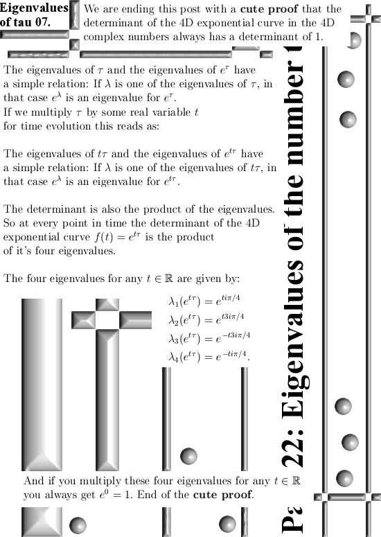
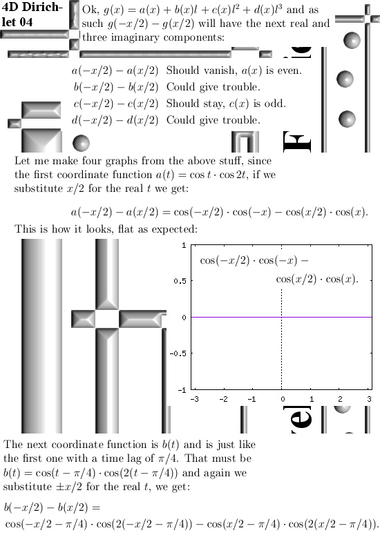
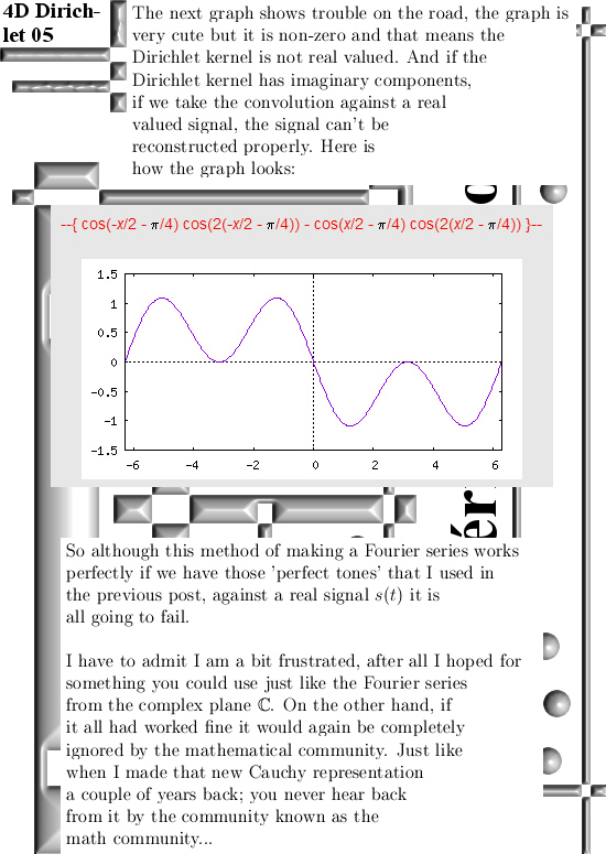
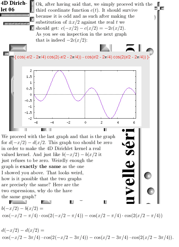
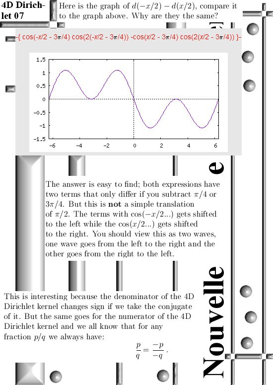
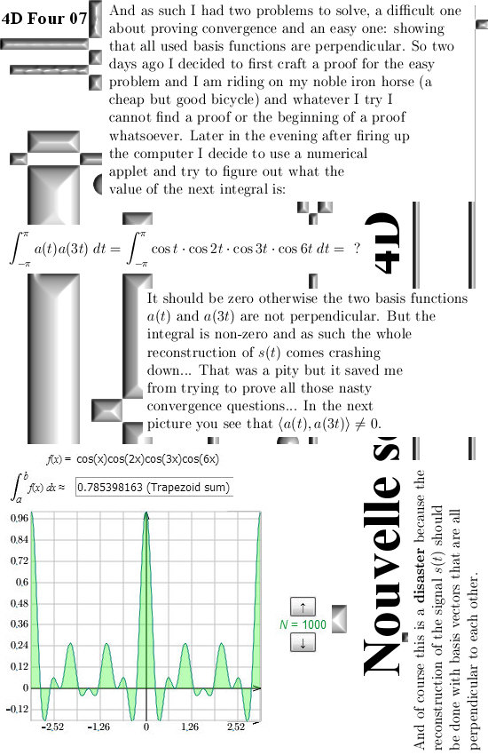
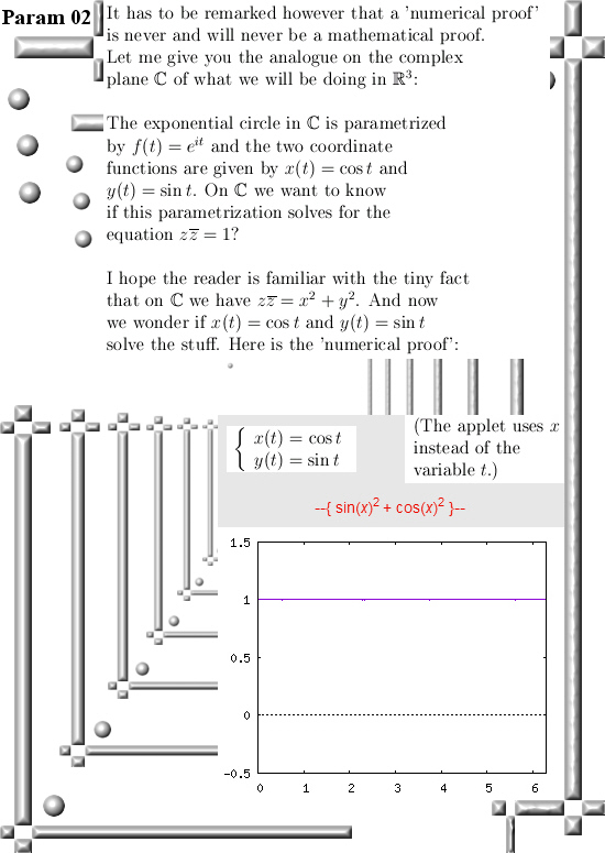
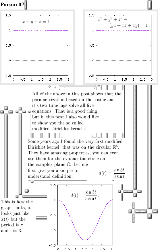
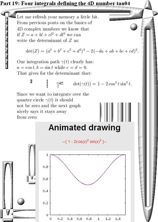
All that’s left for me to do is to hang in the seven images that make up the math kernel of this post. I made them a tiny bit higher this time, the sizes are 550×1250. A graph of the hyperbolic version of the complex exponential can be found at the seventh image. Have fun reading it and let me hope that you, just like me, have learned a bit from this conjugate stuff.
The picture text already starts wrong: It’s five spaces, not four…
At last I want to remark that the 2D hyperbolic complex numbers are beautiful to see. But why should that be a complex exponential while the split complex numbers from the overpaid math professors does not have a complex exponential?
Well that is because the determinant of the imaginary unit must be +1 and not -1 like we have for those split complex numbers from the overpaid math professors. Lets leave it with that and may I thank you for your attention if you are still awake by now.