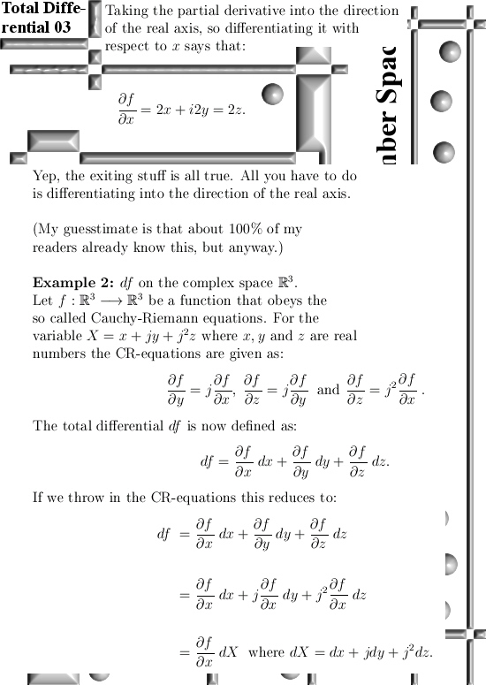
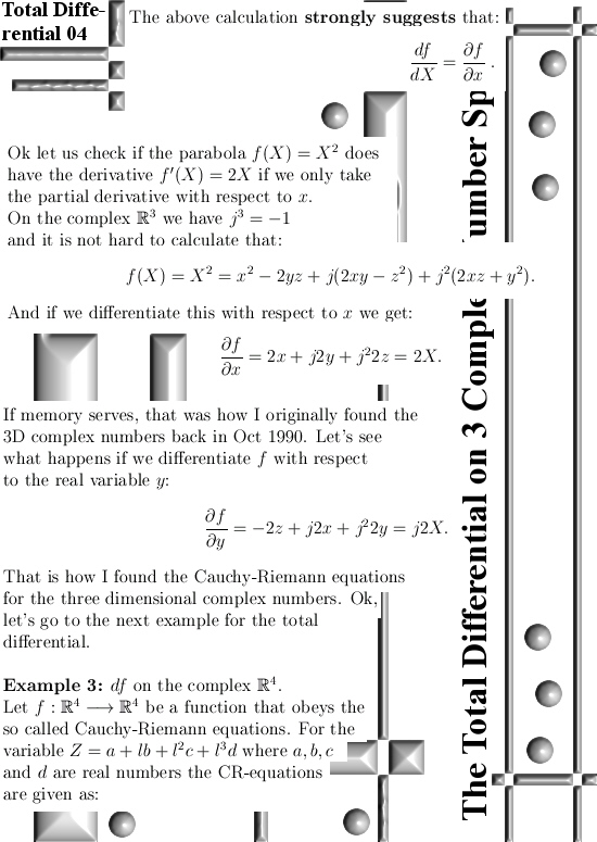
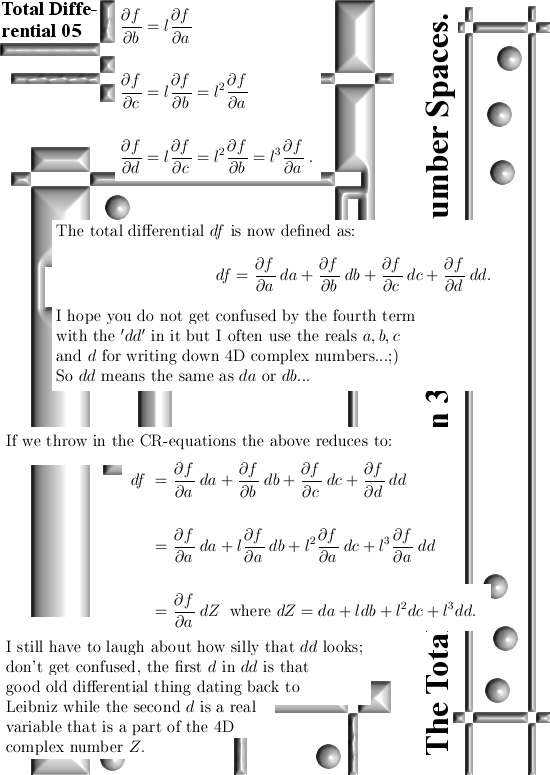
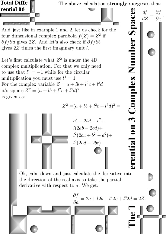
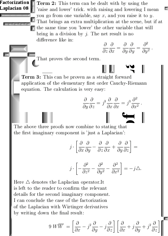
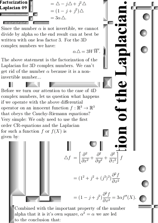
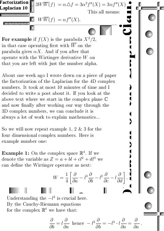
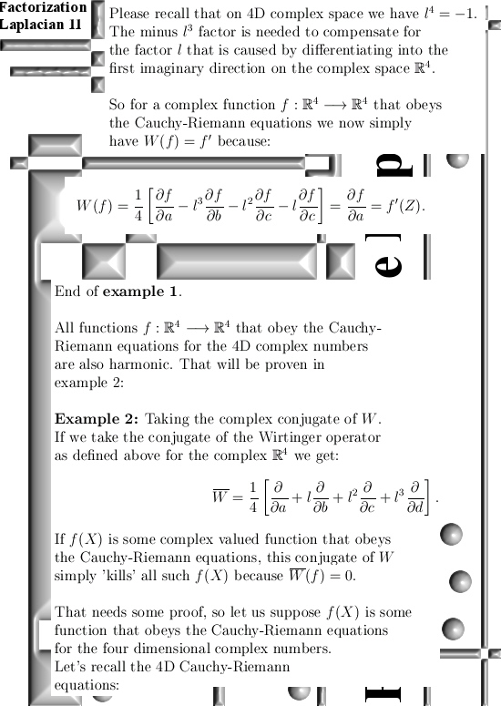
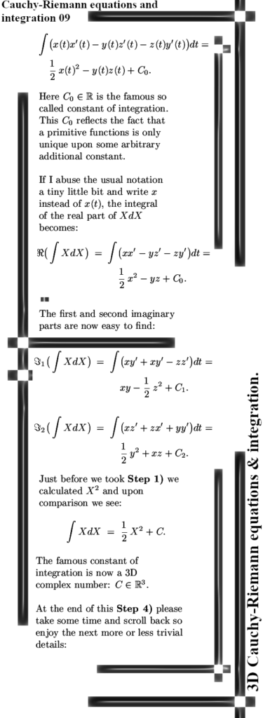
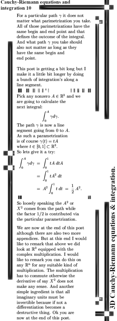
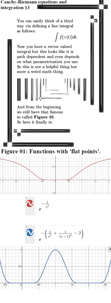
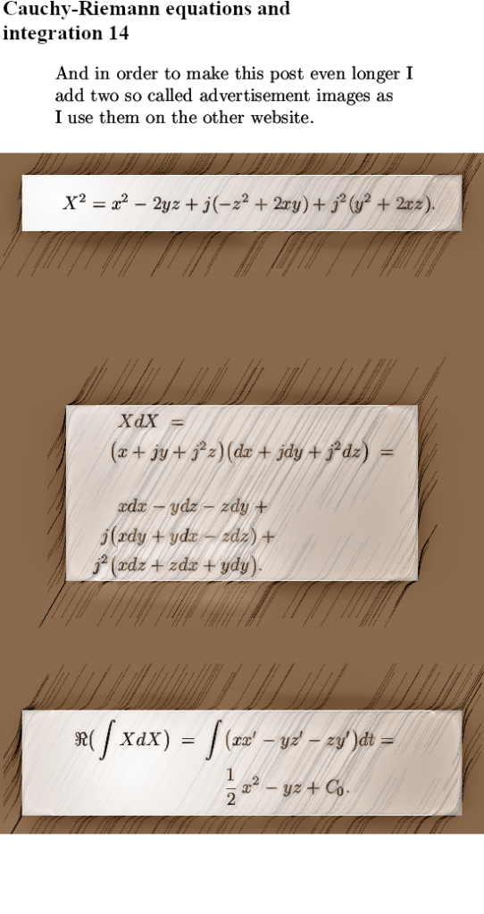
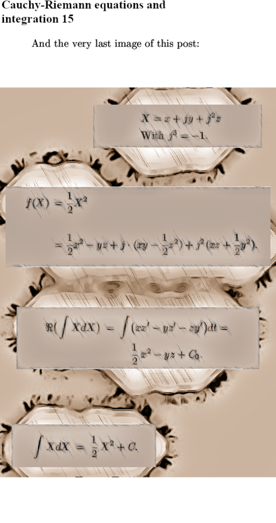
This post is about the CR equations for the 3D complex numbers, as an example we look at the next simple function there is after linear functions: the square. On us will fall the noble task of differentiation 0.5X^2 on the 3D complex numbers and of course we will find the identity function. To top it all off, after that we integrate the identity function with respect to X, so we evaluate XdX and miracle miracle we get 0.5X^2.
So more basic as this is not possible, only boring stuff like how to add two 3D complex numbers is even more basic. And for me it was actually fun to write it down one more time after so many years. Also as far as I remember, I never had differentiation and integration in one post combined. Mostly I treated them separately.
Because this subject was so elementary I allowed myself for one time to not skip a lot of stuff. Just pen down whatever crossed my mind. As a result this post is now 15 images long and I guess that is a decade long record at least.
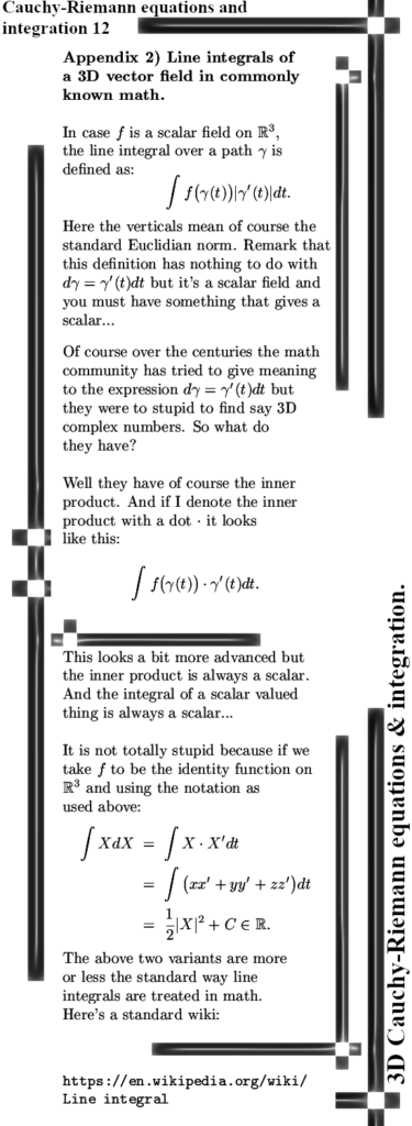
I also included a link to a wiki about line integration in say 3D in order to demonstrate it clearly that the entire math community still can’t do a line integration in 3D using the good old concept of a primitive. Just like we integrate on the real line and the complex plane. After a third of a century of time, those people still have no clue at all. If I remember it all correctly, it is so long ago, it was in 1991 or may be 1992 I found these results. But the local professors here at the university of Groningen did not want to look at stuff like this. That’s how they do science over here…
Anyway the math part is 13 images long and I included two so called advertisement images as I use them on the other website. Ok lets now turn to the 15 images:
That was it more or less for this post. The previous post about circular photons and magnetic domains was a number one search result on Google within 24 hours! Now you must not think I am looking at my search ratings all the time, actually I almost never do that may be less as once a year I don’t know. But I had sought only once on “Circular light and magnetic domains” that just one day after the publishing of the last post I decided to take a look again. And to my surprise my own post on it was the no one result. And ok ok, my search text was more or less precisely the title of my post but on number one in about 20 hours of time?
You also must not jump to the conclusion that a most on the magnetic properties of an electron so fast at number one will make a dent in the attitude of the physics people at universities. My estimation is that they will keep on pretending that electrons are more or less tiny magnets. And just entertaining the idea that magnetic properties and electric properties of electrons are the same so monopole and permanent is just bad for their career. Just as the math profs do with say this post for the last 35 years. Never forget you are dealing with university people and that means most of the time it is more ego and not much science…
With that it is time to end this post and may I thank you for your attention to the matter of line integration in 3D complex space using a primitive?