I made another math post with only differentiating the square function and integrating the identity function like in integrating zdz on the complex plane. This post is much shorter, only 7 images long and one appendix so all in all 8 images. One of the reasons I decided to write another post on this relative simple stuff is that historically speaking the square was the thing that gave the complex plane. And for some reason professional math people are completely fixated on that when they try for example find 3D complex numbers: It has to be based on some stuff with a square. Just like say the 4D quaternions from Hamilton: Basically it’s all based on the squares of the three imaginary components and an extra rule for multiplying different imaginary units.
Without much ado let me hang in the 8 images:
It is no secret that inside the profession of math at the universities they can only perform integration with a primitive when it comes to the real line and the complex plane. In the last two posts I showed you again and again how to do this on other spaces. Will the professional community ever change ways and include more spaces where you can perform integration ‘Just like on the real line’? No, after all these are university people and as such it is mostly a giant balloon of hot ego air and not much substance when it comes to math.
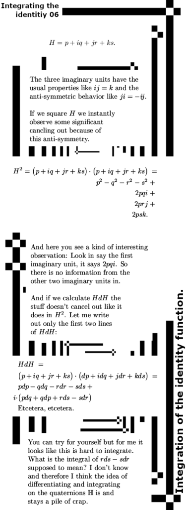
By accident I came across a work of professor Tom who happily informs his audience of the miracles of the 4D quaternions. You know for me math is a hobby, it’s an important hobby but it’s just a hobby. And because after all the subject is math I take it seriously. But decade in decade out the only thing professional math professors do is fuck around and that’s it. Here’s the link to the garbage from professor Tom: Stop 3: Multi-dimensional World These people just never make any kind of progress, if it’s the year 1990 or the present 2026 it just does not matter. They can’t go beyond the square and also they are very unwilling to go beyond the square. Let me leave my little rant with that, here’s what missing in literally all texts on quaternions: The square of a quaternion…
Ok that was it for this latest post. Likely the next post is one on magnetism in particular electron pairs in chiral molecules. Thanks for your attention.
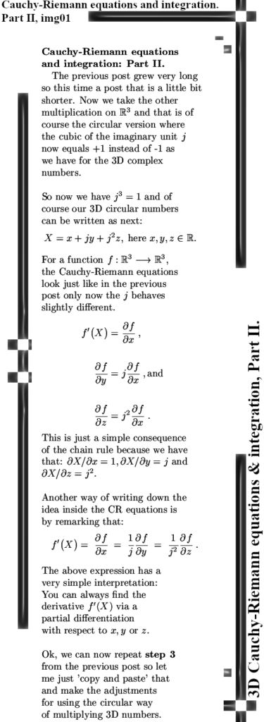
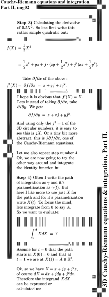
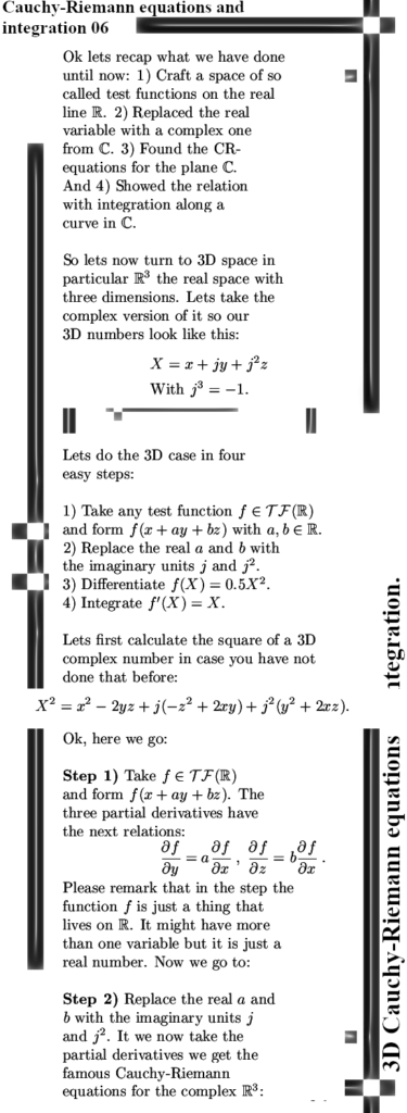
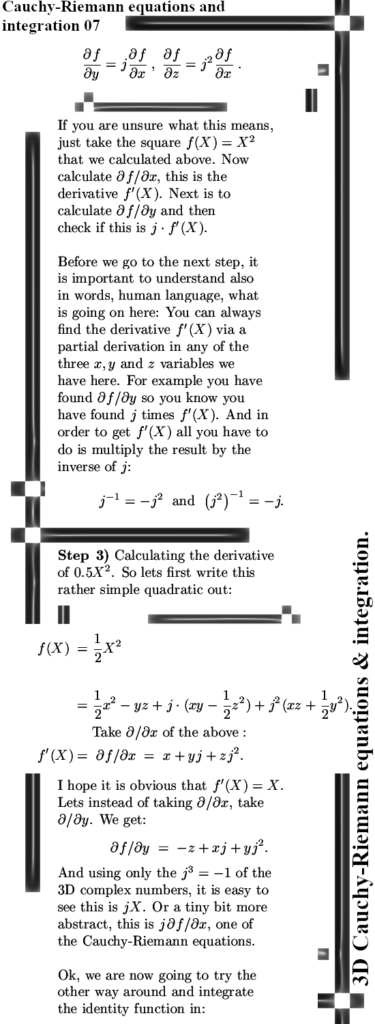
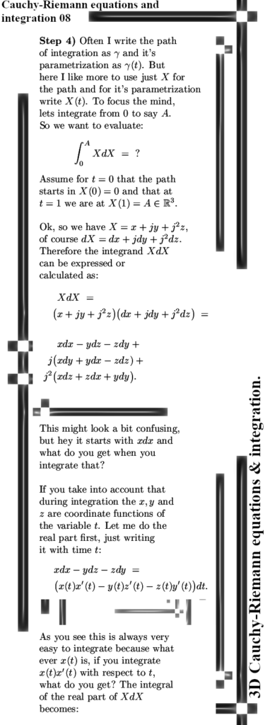
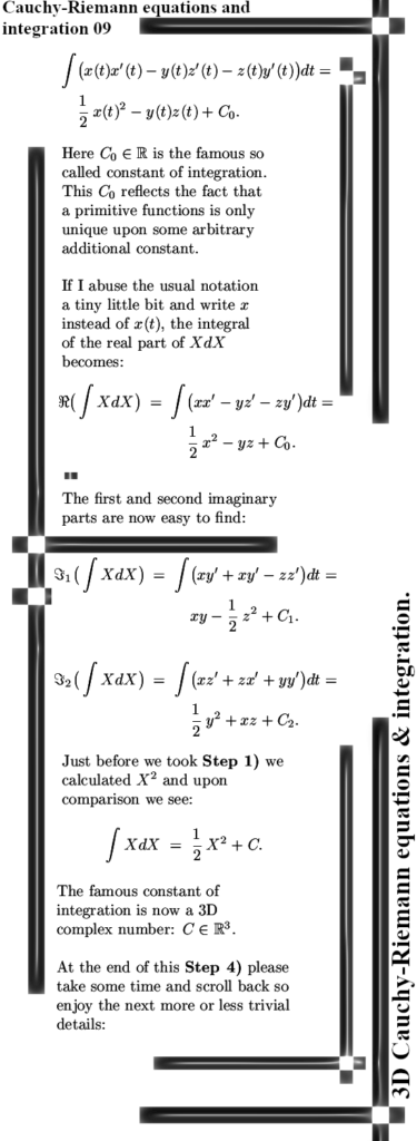
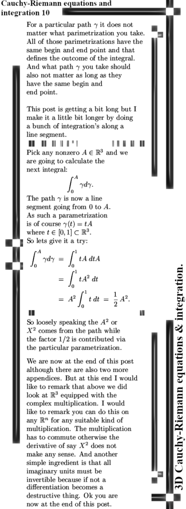
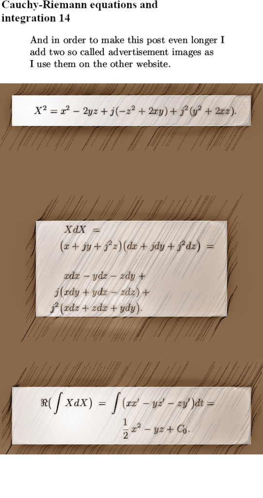
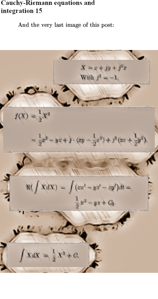
This post is about the CR equations for the 3D complex numbers, as an example we look at the next simple function there is after linear functions: the square. On us will fall the noble task of differentiation 0.5X^2 on the 3D complex numbers and of course we will find the identity function. To top it all off, after that we integrate the identity function with respect to X, so we evaluate XdX and miracle miracle we get 0.5X^2.
So more basic as this is not possible, only boring stuff like how to add two 3D complex numbers is even more basic. And for me it was actually fun to write it down one more time after so many years. Also as far as I remember, I never had differentiation and integration in one post combined. Mostly I treated them separately.
Because this subject was so elementary I allowed myself for one time to not skip a lot of stuff. Just pen down whatever crossed my mind. As a result this post is now 15 images long and I guess that is a decade long record at least.
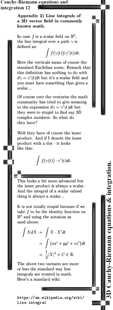
I also included a link to a wiki about line integration in say 3D in order to demonstrate it clearly that the entire math community still can’t do a line integration in 3D using the good old concept of a primitive. Just like we integrate on the real line and the complex plane. After a third of a century of time, those people still have no clue at all. If I remember it all correctly, it is so long ago, it was in 1991 or may be 1992 I found these results. But the local professors here at the university of Groningen did not want to look at stuff like this. That’s how they do science over here…
Anyway the math part is 13 images long and I included two so called advertisement images as I use them on the other website. Ok lets now turn to the 15 images:
There was a typo in the image, now 02 May it’s repaired.
That was it more or less for this post. The previous post about circular photons and magnetic domains was a number one search result on Google within 24 hours! Now you must not think I am looking at my search ratings all the time, actually I almost never do that may be less as once a year I don’t know. But I had sought only once on “Circular light and magnetic domains” that just one day after the publishing of the last post I decided to take a look again. And to my surprise my own post on it was the no one result. And ok ok, my search text was more or less precisely the title of my post but on number one in about 20 hours of time?
You also must not jump to the conclusion that a most on the magnetic properties of an electron so fast at number one will make a dent in the attitude of the physics people at universities. My estimation is that they will keep on pretending that electrons are more or less tiny magnets. And just entertaining the idea that magnetic properties and electric properties of electrons are the same so monopole and permanent is just bad for their career. Just as the math profs do with say this post for the last 35 years. Never forget you are dealing with university people and that means most of the time it is more ego and not much science…
With that it is time to end this post and may I thank you for your attention to the matter of line integration in 3D complex space using a primitive?
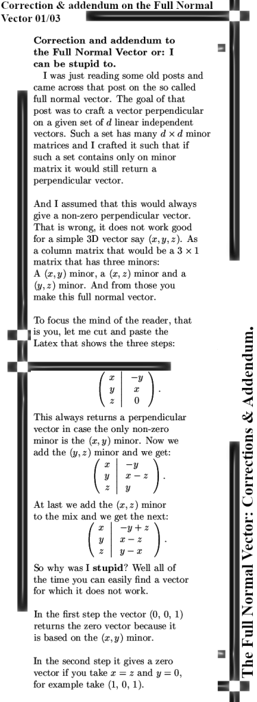
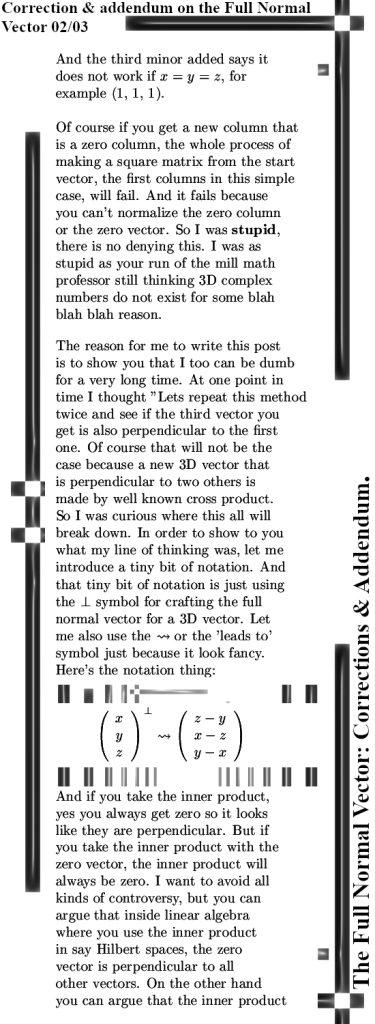
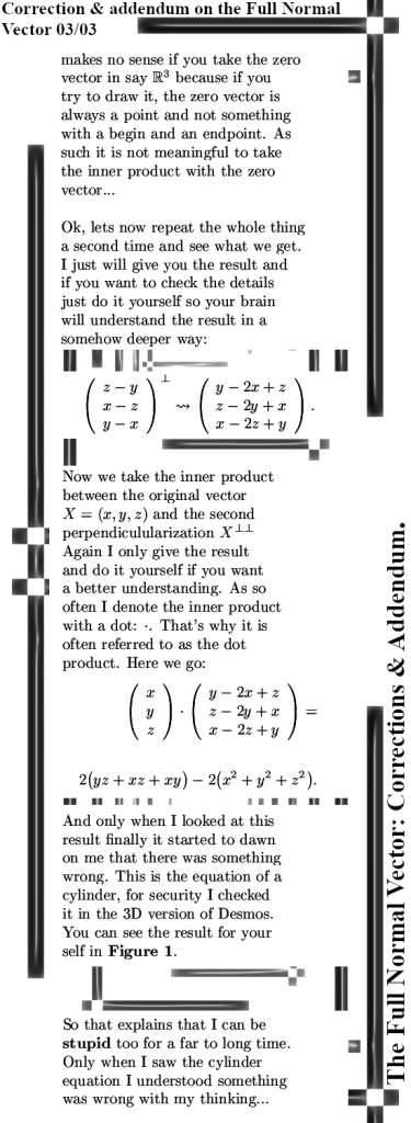
Some time back I was looking at a few recently published posts and I started scribbling a few calculations. And all of a sudden I realized something has gone wrong. Now that full normal vector does what it was supposed to do: Always return a normal vector even if there is only one minor matrix that is not singular. But sometimes you get a zero vector and that is not what you want of course. You can always work around it if it happens to you, so it is not a serous fault or so. But it’s all a tiny bit less perfect as I thought.
That full normal vector is something you can use if you want to make a non square matrix into a square one. In doing so you must craft new columns perpendicular to all previous columns and normalize them. And there is the problem of course: If you get a zero vector, you cannot normalize it to length one.
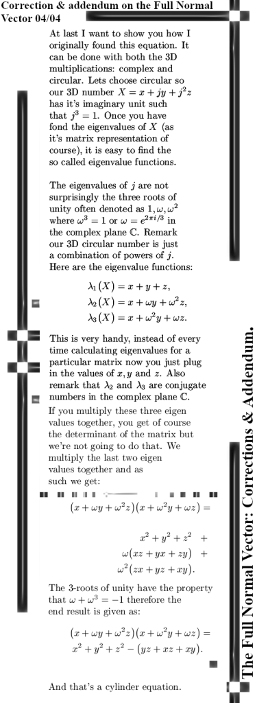
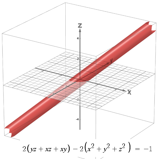
The reason I decided to write this post is that during my scribbling I soon got one of those cylinder equations that don’t look at all like the equation of a cylinder. But in the 3D numbers, both complex and circular, you can factorize the determinant with a plane and a cylinder equation. So in that sense it is very vaguely related to the 3D numbers. For 3D numbers you can factorize the determinant using it’s eigenvalues and stuff like that I always name “Eigenvalue functions” because you just plug in the coordinates of a number and voila: There are your eigenvalues. It’s much easier compared to every time by hand calculating the 3 eigenvalues every 3D number has.
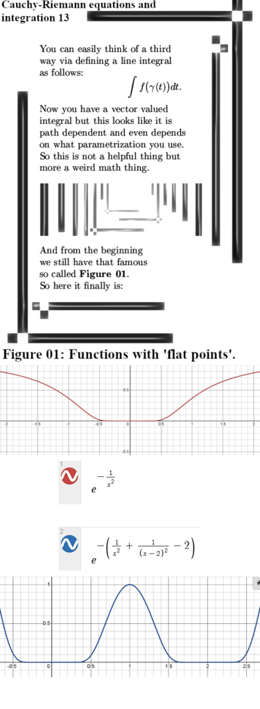
This post is four images long and an extra graph in a so called “Figure 01“. With the 3D version of Desmos, a free browser based app for drawing graphs, you can try a bit for yourself. I used two versions of the cylinder equation, don’t get confused by that because the one is only the minus of the other. That’s why in Desmos you sometimes must equal the cylinder equation to a positive number or a negative number. Here we go:
Again: If you try it in Desmos you must either use positive or negative numbers for your cylinder equation.
In case you want to know a bit more about the eigenvalue functions, just use the search function of this website and you will find plenty of stuff to think about. Ok, I hope you learned something and if not lets hope you are not one hundred % bored because math is just a boring thing or not? The next post is likely about magnetism but it is also tempting to write one more post on all the possible factorizations you can do with the determinant of 3D numbers and the many ways there are to find the 3D complex exponential as the intersection of a whole lot of geometrical objects. We’ll see.
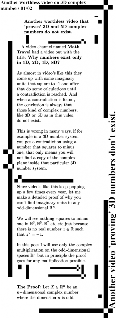
This year a couple more video’s were published on youtube regarding this subject of the non-existence of 3D complex numbers but I skipped those and did not comment a thing. So why this video? Well those ‘proofs’ always have some things in common namely the idea that there are imaginary units in say 3D or 5D space that square to minus one. And after that those people do some calculations or math manipulations, find something that contradicts and voila the conclusion is: 3D complex numbers do not exist. Some people, but not many, are a bit sharper by stating this proofs that there is no 3D extension that includes the 2D complex plane.
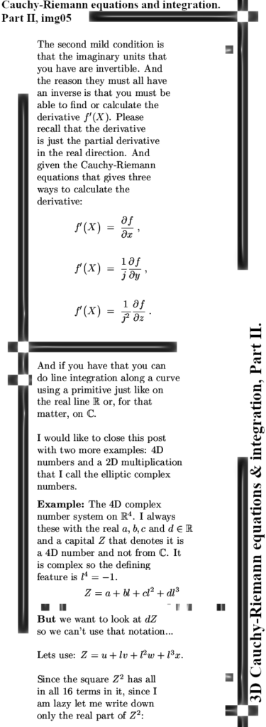
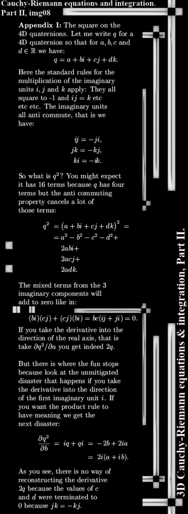
But 3D or 5D or any dimension numbers do exist in there own way. In 3D space there is an imaginary unit who’s third power equals minus one, in 5D space the fifth power is minus one etc etc. And in all of those spaces you can do complex analysis because you can differentiate and perform integration ‘just like’ in the complex plane. As a comparison on those overhyped quaternions you can’t even differentiate the function that squares a quaternion. Those 4D quaternions have their own right of existence but they are not the 4D complex numbers, but I digress.
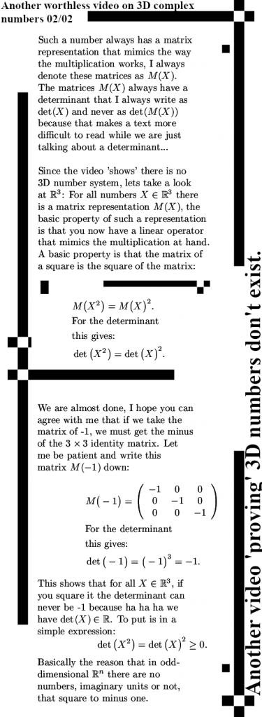
I wrote a very small math post, it is only two images long, with a proof as simple as possible that shows in real spaces with an odd number for the dimension, there are no numbers that square to minus one.
Now we all know that on the real line there is nothing that squares to minus one and in all other higher dimensional spaces if we take the determinant we get always get a real number. As such there is no determinant of any number that squares to minus one. And if you calculate the determinant of -1 (as a matrix in odd dimensions) you always get -1…
The proof below is all utterly simple but it’s relevance lies more into that it now goes for all multiplications in one single strike. So not only the so called complex multiplication but just everything that is a multiplication. If for some strange reason you want to think a bit of what all can pass as a multiplication, just use the search function of this website and search for big E. Big E is just a multiplication table although I present it like a square matrix for reasons that are obvious if you read that post.
At last I want to remark that although the title is a bit negative, I wish the composer of the video good luck with his math travels. That, by the way is the name of the video channel: Math Travel. Let me first post my two images and later the video.
Ok, lets now all smile and wave at youtube so the next video will get shown to you:
Well that was it my dear reader, thanks for making it all to the end with all that boring math stuff and so.
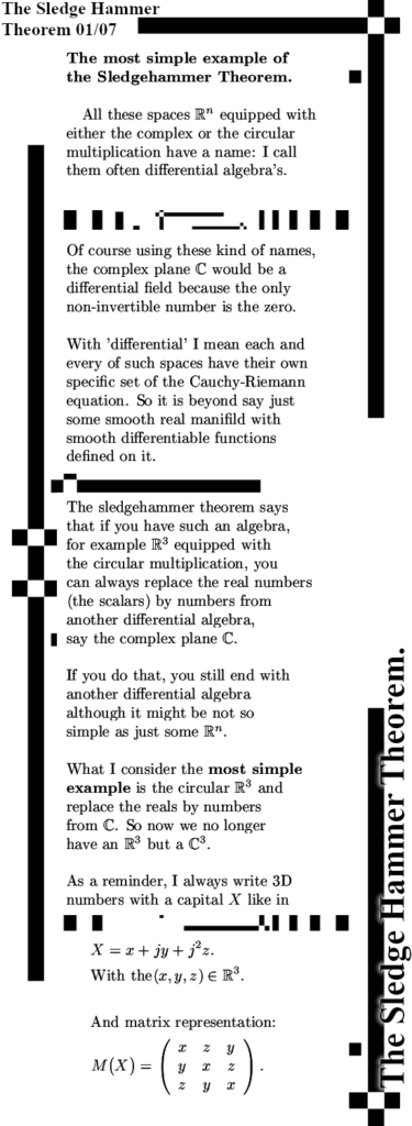
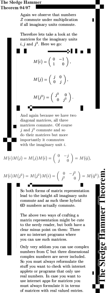
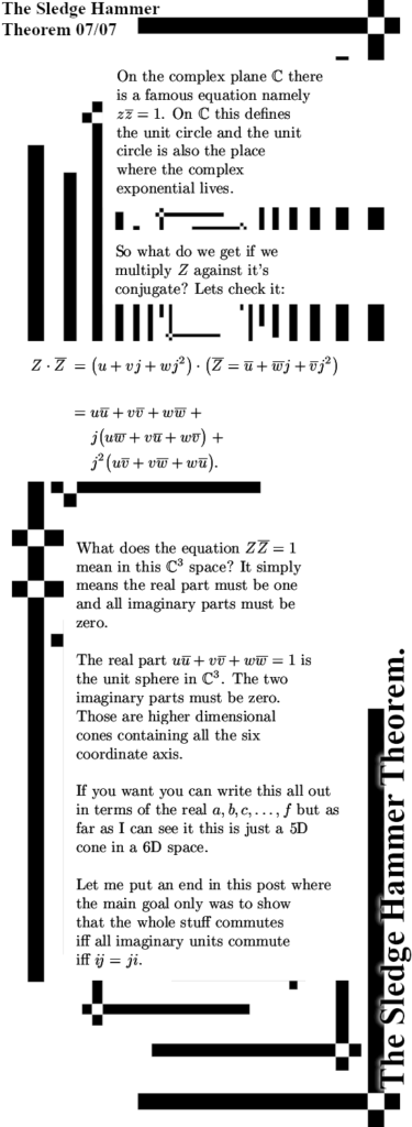
When reading some old texts I found that in the past I named this theorem the Scalar Replacement Theorem and that is may be a better description of the stuff involved. The Sledge Hammer theorem says that if you have say a 3D complex or circular number, you can always replace the reals by numbers from other higher dimensional system. I took the 3D circular numbers, so the third power of the first imaginary unit equals one, and replaced the real x, y and z by the 2D complex numbers from the complex plane. Of course you know that in the complex plane the imaginary unit i squares to minus one so if we replace the reals by 2D complex numbers we get a 6D number system.
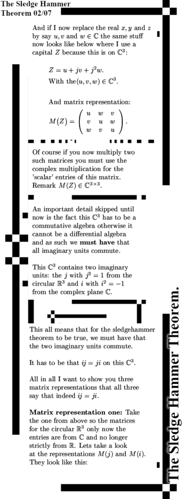
The Sledgehammer Theorem says that if you do that, the newly formed 6D number system commutes and if you want you can find the Cauchy-Riemann equations that belong to this particular set of higher dimensional numbers. This is the very first hybrid number system I crafted, it is hybrid because it is not circular nor complex but has imaginary units that are different in that detail.
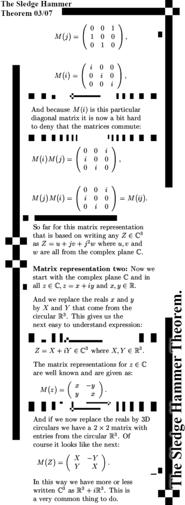
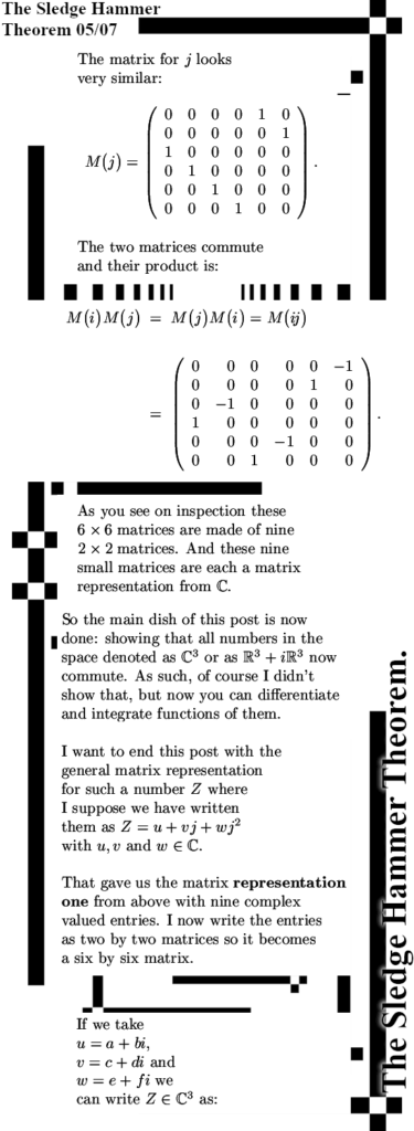
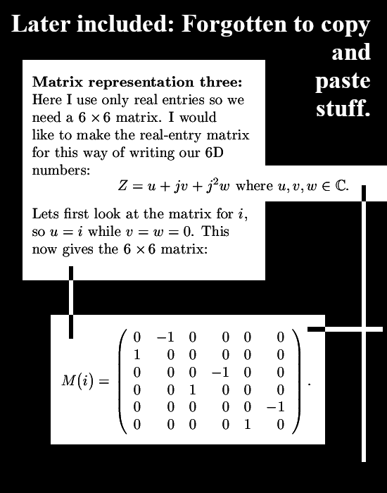
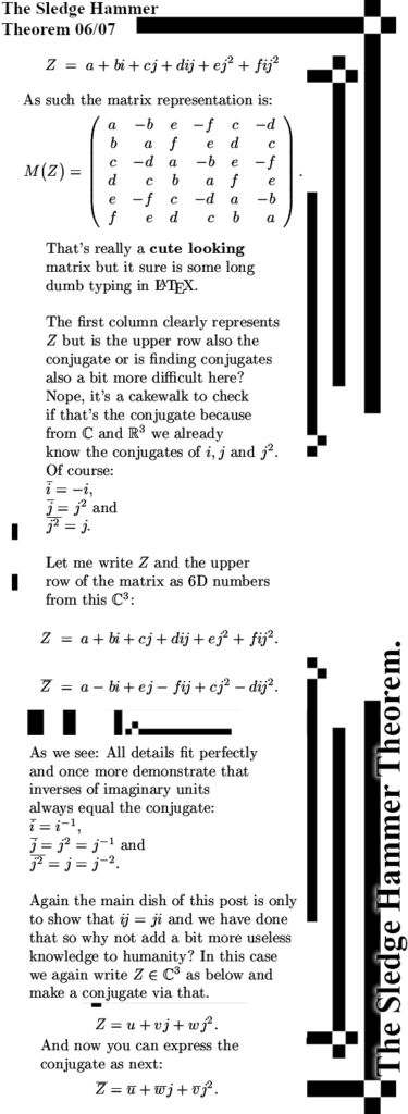
The main goal of this post is to show that both imaginary units commute and that makes the whole 6D number system commute. I concentrated on two different ways of making a matrix representation and I kept it that way. So the simple to understand thing that ij = ji is the main goal of my new post but from experience I know that for other people it is always amazingly hard to find a conjugate. On the complex plane it is just a flip in the real axis and for some strange reason people always do that and end up with rubbish in say spaces like the 3D circular numbers. Therefore I took the freedom to include the conjugate and of course if you have the conjugate why not try to extract a bit of cute math like the sphere-cone equation from it and see how this looks in this 6D hybrid number system.
The post is seven pictures long and one appendix so all in all eight pictures of size 550×1500 pixels. I tried to keep it all as simple as possible but hey it’s a 6D space made from a 3D circular space and a 2D complex space. Have fun reading it.
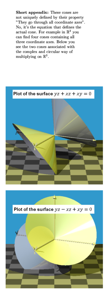
And I made a tiny appendix upon those cone like structures. Only in 3D it is a proper 2D cone of course. It is only to show that a cone is defined by it’s equation and it has the property it goes through all coordinate axes. Even in 3D space there are four cones that include all coordinate axes, I show you the cone associated with the complex and circular 3D spaces.
That was it for this post that despite it’s rather limited math content grew a bit long after all. In case you haven’t fallen asleep right now may I thank you for your attention. May be we do a good old post on magnetism as the next post or just somehting else. I don’t know yet so we’ll see.
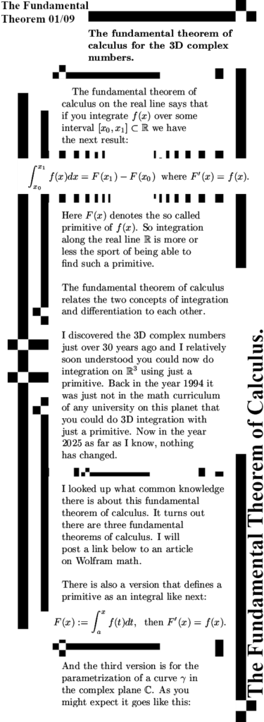
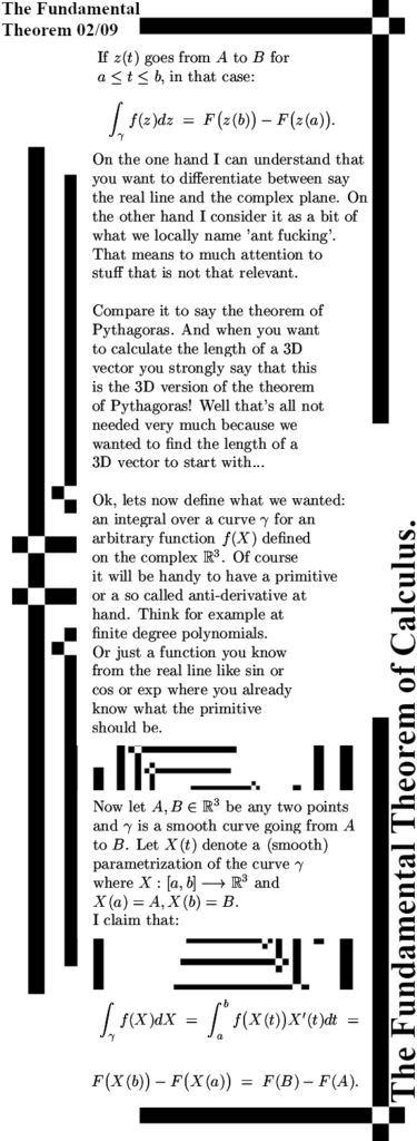
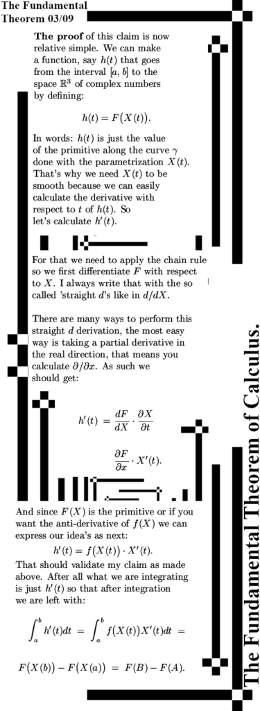
Some time after I started writing this post I thought “Hey why not look up what is more or less offically said on this theorem in the internet”. So I did and found out there are three versions of this theorem that basically says you can do integration with a primitive. That was a tiny surprise to me because the way I remembered it was there is just only one. There are two versions on the real line and one for the complex plane. The first real line version says that the integral of a function on the real line equals the difference that the primitive has in the begin and endpoint of integration. The second real line version uses a variable in the endpoint of integration, say x, and define a primitive F(x) of a function f(x) as such. After that it must be shown that the derivative F'(x) = f(x). And the third version says you can do line integration (or integration along a curve traditionally named gamma) also using a primitive but now you must take into account the way differentiation works in the complex plane.
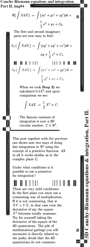
So there is not one such fundamental theorem but the official theory says it’s three. Now why three? Very simple: The professional math people know of no other spaces where you can do integration with a primitive. I’ve said it before and repeat it once more: The 4D quaternions are nice things but when it comes to differentiation and integration it is hard to get a bigger mess of total gibberish. That’s why the professional math professors don’t have such a fundamental theorem for the quaternions.
But for the 3D complex numbers that are the main topic of this website, it can also be done. But hey this is now the year 2025 and this website is almost 10 years old and on top of that I found the 3D complex numbers back in the year 1990, so why only now this theorem in the year 2025? Now over the years I have always used this kind of integration when I needed it. For example the number tau for the 3D complex numbers was calculated the first time by using integration while I developed the matrix diagonalization methods only later to deal with the problems you get in say five or seven dimensional complex numbers. For people who don’t have it clear what the numbers tau are: They are the logarithm of an imaginary unit. For example the log of the imaginary unit i on the complex plane is i times pi/2 as was already found by the good old Euler. Now for the 3D complex numbers it’s a bit more difficult but you can find such log’s of imaginary numbers indeed with integrating just the inverse.
But I always thought there would be some kind of trouble if you integrate just inside the subspaces of non-invertible numbers. So that’s more or less why I never ever formulated such a fundamental theorem in all those years. I only used integration when I needed it and that was it.
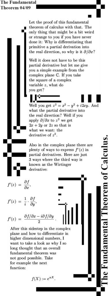
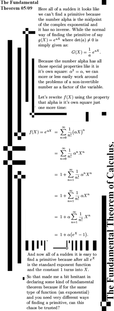
To my excuse there are indeed some subtilities, I once tried to find the primitive of say e^X and yes, no problemo, it is just e^X. While if you calculate the integral now with a 3D number X but multiply it by that famous number alpha, the primitive changes in a dramatic fashion. So all those years I thought that even for say the exponential function there was not just one primitive to do all the work. Yet now I take a deeper look into it, this was all a bit stupid of me. So it’s a lame excuse but compared to the professional math professors who can’t even find the complex 3D numbers, I shine as the stable genius I am… Ahum, this post is only 9 pictures long and has 3 additional figures and one video about the fundamental theorem on the real line. So all in all there are 12 pictures and 1 video below.
Lets get this party started:
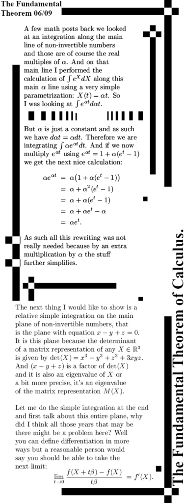
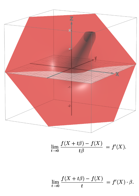
The next picture is the so called Figure 1 picture and it shows where the determinant is one. So on the red colored graph you can do the ‘divide by beta’ thing in the limit for the derivative of a function. The problems with taking such a limit on the space where det(X) = 0, you can’t divide by such a beta so doesn’t that cause some problems? Well no, you can always flip hin und her between the two above definitions of taking a derivative.
Figure 1: I am not crazy: Can’t divide by beta? Well, try a multiplication by beta…
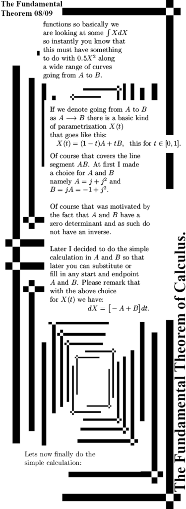
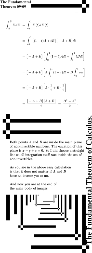
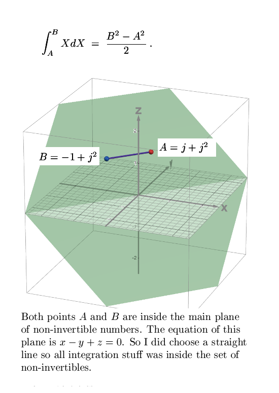
And here is the so called Figure 2 picture where I depicted a line segment inside the main plane of non-invertible numbers in the 3D complex numbers. Therefore I invite you to think a bit along those lines, does it matter if they are inside or outside the space of det(X) = 0?
I have a link for you to a page from the website from Stephen Wolfram where the three fundamental theorems of calculus are explained. Fundamental Theorems of Calculus Now I published the above about 24 hours ago but I was forgotten to place the link to Wolfram. And today I was watching youtube and to my surprise a video from Hannah Fry came floating along while it said it was about the fundamental theorem of calculus. It’s all very very basic because Hannah uses it also to craft an introduction to integration using the limit of an elementary Riemann sum. For most readers it is a bit too simple I guess but in case you harldy know what integration is, for those it is a very good video.
And for no reason at all I also made a cube with her face on it. We all love Hannah because she is relatively good at popularizing math. And that’s a good thing because it makes the general population a bit less stupid. Anyway that is what you might hope for but don’t let you hope become to big because the human brain and math is often not a good combination. We’re just a fucking stupid monkey species, ok we are the smartest monkeys around but we’re still a monkey species…
This is the end of this post, now we have a fourth so called Fundamental theorem of calculus. Lets leave it with that.
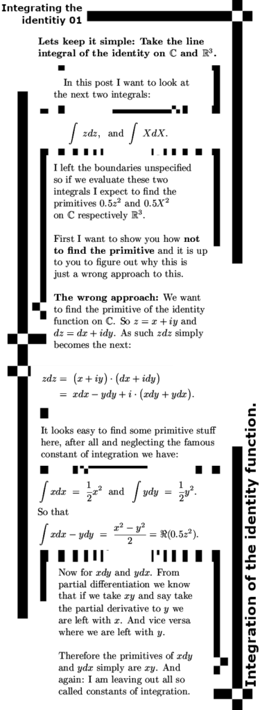
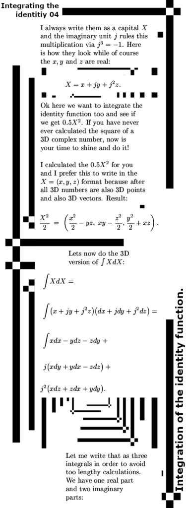
This is now post number 278 on this website and to be honest the content of this post should have been here years ago. This post is about complex integration and I more or less compare how you do that in the complex plane against how it is done in 3D space. Integrating the identity simple means integrating zdz on the complex plane and XdX on the space of 3D complex numbers. Of course I have used complex integration in higher dimensional spaces in the past when I needed it. For example this is how I found my first number tau: On the space of 3D complex numbers you must find the logarithm of j^2 (not j because j has a determinant of minus one) and I did that with complex integration. For people who are new to this website: j denotes the imaginary unit in 3D space and it’s third power equals -1. That mimics the situation in the complex plane where the imaginary unit i if you square it that gives -1.
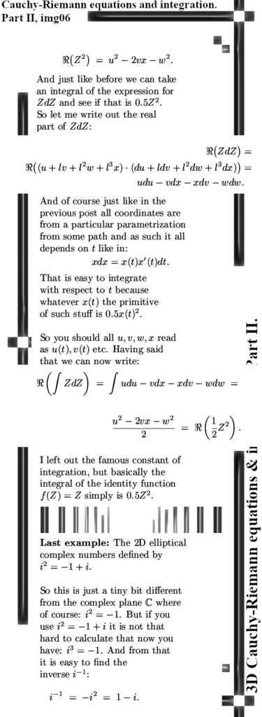
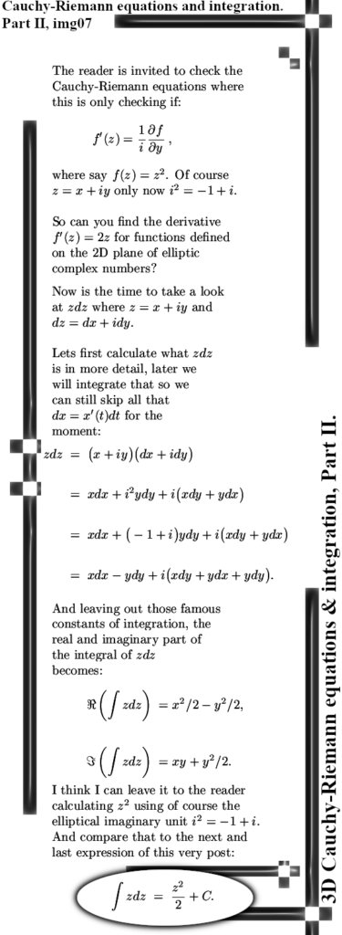
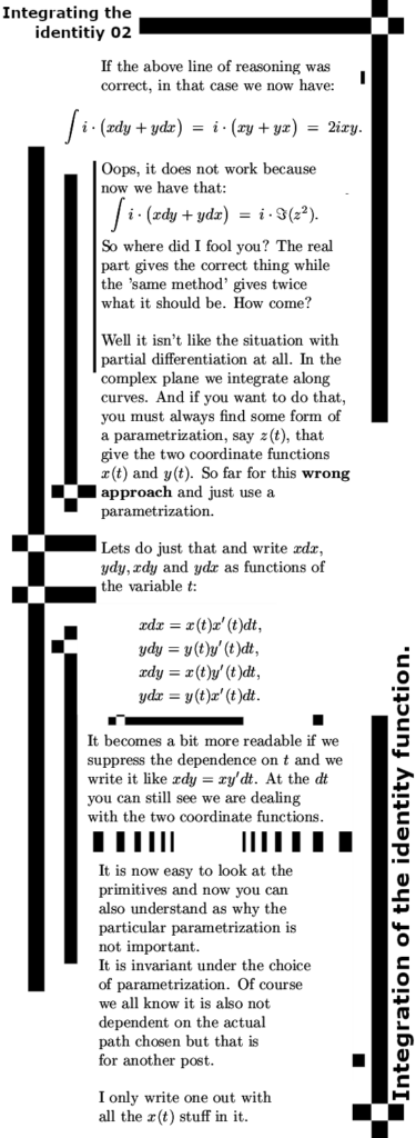
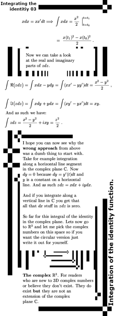
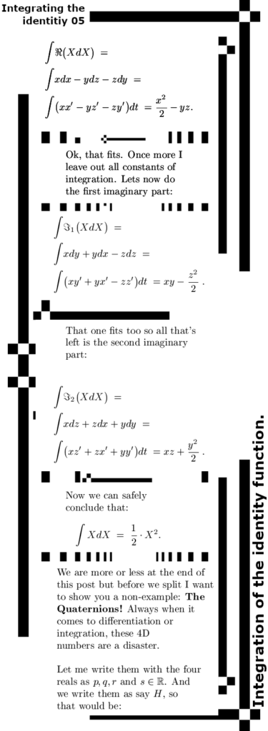
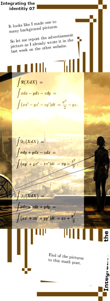
All these years I never used complex integration just to find a primitive, so that is done in this post. And since we are integrating zdz we expect to find 0.5z^2on the complex plane while on my beloved space of 3D complex numbers the integral of XdX should yield 0.5X^2. Of course we will find these results because otherwise I would have been very stupid in say the last 15 years. Of course just like every body elso I have been very stupid on many occasions on such long timescales, but not when it comes to 3D complex numbers.
Oops, I see I still have to make the seven png pictures but that won’t take very much time. So that’s this math post: 7 pictures of each 550×1500 pixels in size. I hope that after reading it you can also perform complex integration is say the space of 4D complex numbers. And now we talk about 4D numbers; I also included at the end the famous quaternions and of course if we try to integrate them we get the usual garbage once more demonstrating that when it comes to differentiation and integration the quaternions are just awful.
That was it for this math post. Likely the next post is another video where the famous Stern Gerlach experiment is explained. Of course in such videos they never jump to the correct conclusion that says it is very likely that electron magnetism is monopole in nature. Just like their electric charge by the way, of course for all professional physics persons the electron has to be a tiny magnet. Not that they have much so called ‘five sigma’ experimental evidence for that, but for them this is not a problem…
Ok, let me hit that button ‘publish website’ and may I thank you for your attention.
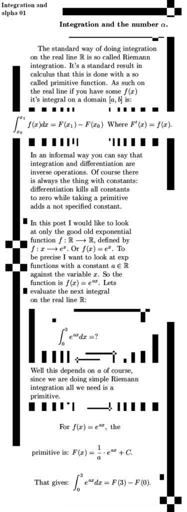
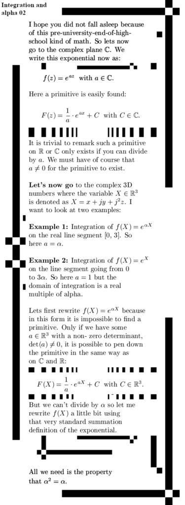
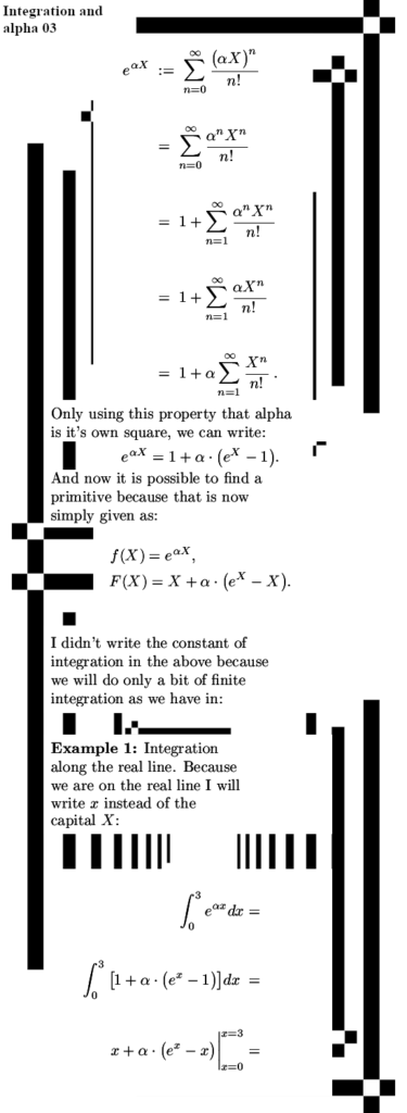
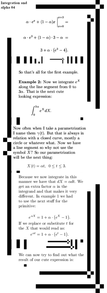
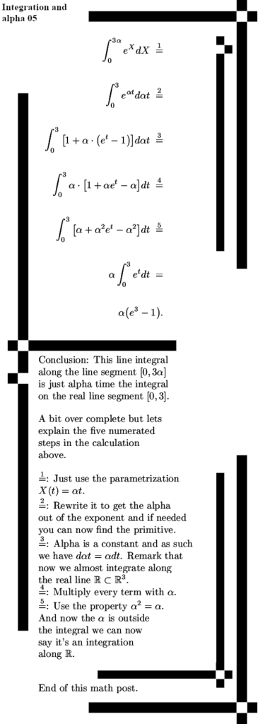
It’s about time to write this post because the pictures were finished a few days back but I was a bit lazy in the meantime. In this post I only evaluate two line integrals both in some way related to the famous number alpha. And we do it only on the 3D space, there are much more numbers alpha on other spaces but we just do the complex and the circular multiplication in three dimensions. In this post when it comes to the number alpha we mostly need the one property that alpha is it’s own square. Therefore you can break down all powers of alpha into alpha itself, this is very handy when for example you use a power series. As always X denotes a 3D number and one of the integrals we will look at is the exponential of alpha times X: exp(alpha * X). Why do we do this? Well try to find a primitive of the above exponential, that is a bit hard because another property of alpha is that it has no inverse and as such you can’t divide by alpha and so what to do? The second example is integration of the most standard exponential exp(X) along the main axis of non-invertibles: All real multiples of the number alpha. For me this was a surprising result because it all becomes so much more simple. All in all this post is five pictures long but it is in the 550×1500 pixel size so they are relatively long. Ok that is all I had to say and let me now hang in the five pictures:
That was it for this post, thanks for your attention and may be see you in a future post.
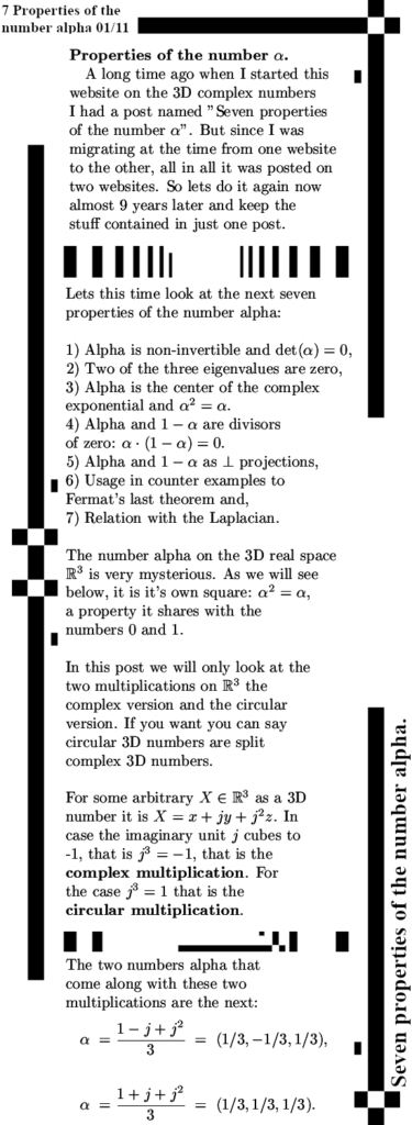
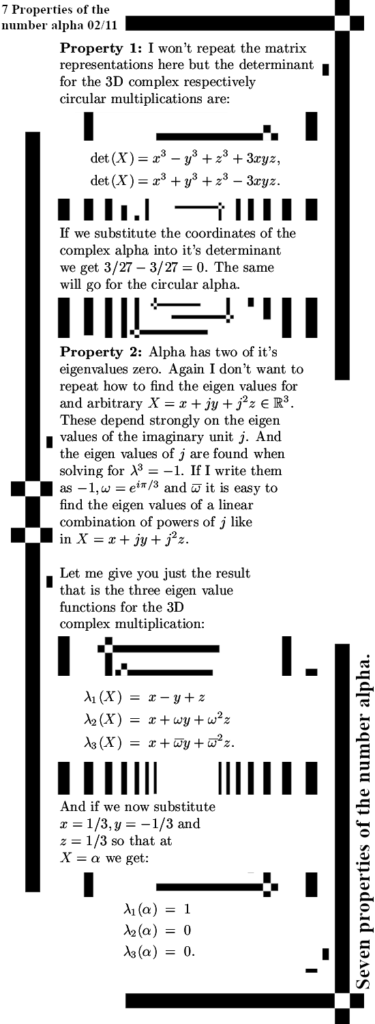
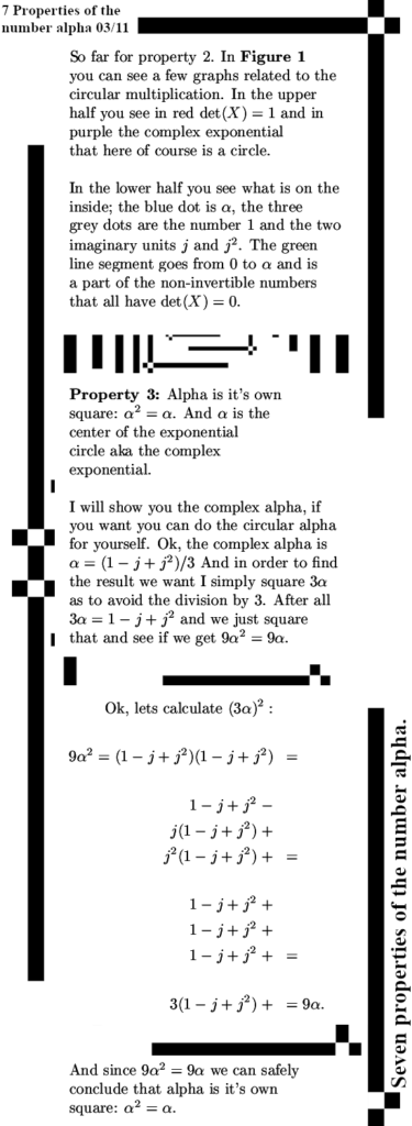
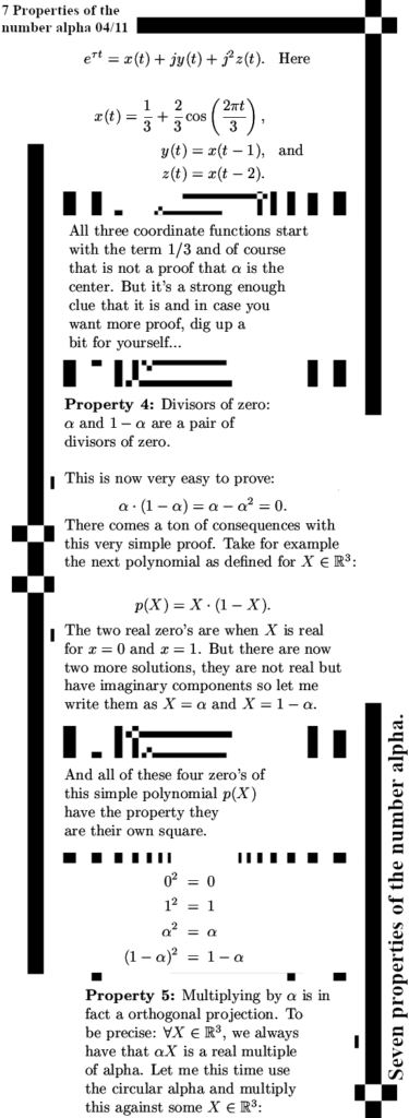
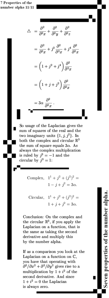
A long time ago around the time I started this website I had something known as “The seven properties of the number alpha”. But it was all spread out over two websites because until then I wrote the math just on the other website. But over the years I have advocated a few times to look up that stuff as the seven properties of alpha, so I decided to write a new post with the same title. I didn’t copy the old stuff but just made up a new version. The post is amazingly long; a normal small picture has the size of 550×775 pixels, larger ones I use are up to 550×1100 but now it has grown to 11 pictures of size 550×1500. Likely this is the longest post I have written on math ever. As always I have to leave a lot out, for example doing integration with the involvement of the number alpha is very interesting. During writing I also remembered that e to the power pi times i times alpha, wasn’t that minus one? Yes but we are not going to do six dimensional numbers or hybrids like the 3D circular numbers and replace the reals by the 2D complex numbers. Nope, in this post only properties from the 3D numbers alpha; the complex and the circular one. More or less all the basic stuff is in this post; from simple things like alpha has no inverse to more complicated stuff like the relation with the Laplacian operator. I made a new category for this post, it even has the name “7 Properties of Alpha” so that in the future it will be even easier to find.
Lets hope it is worth of your time and lets hope you will find it interesting.
Figure 01: Alpha is the center of the complex exponential.
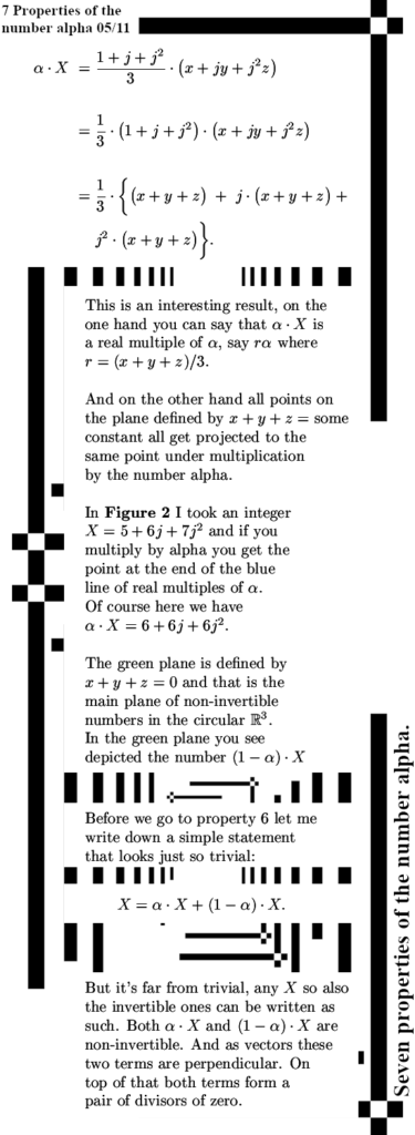
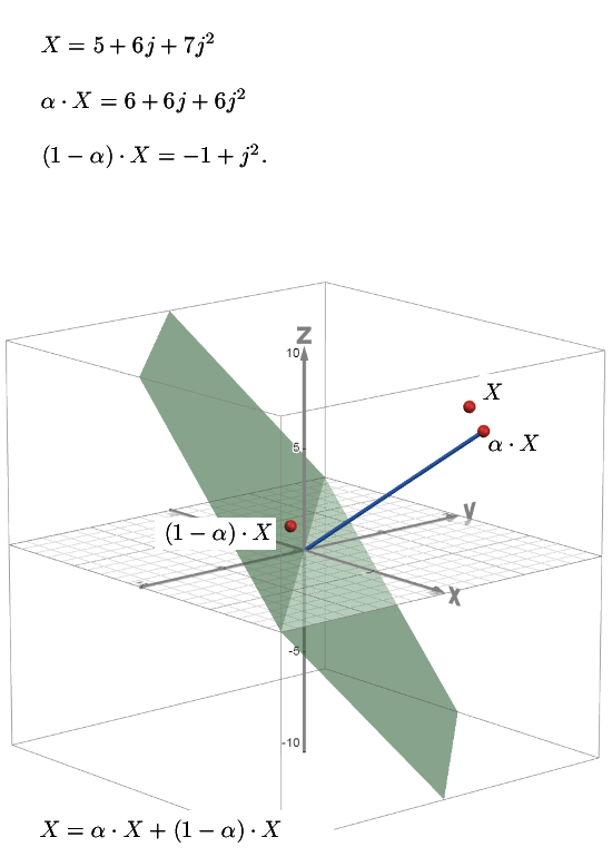
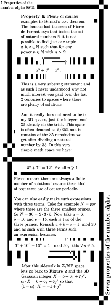
Figure 02: You can write X as the sum of two non-invertible numbers.
Ok, that was a long read. I want to congratulate you with not falling asleep. I have no plans for a next post although it is tempting to write something about integration along the line of real multiples of the number alpha.
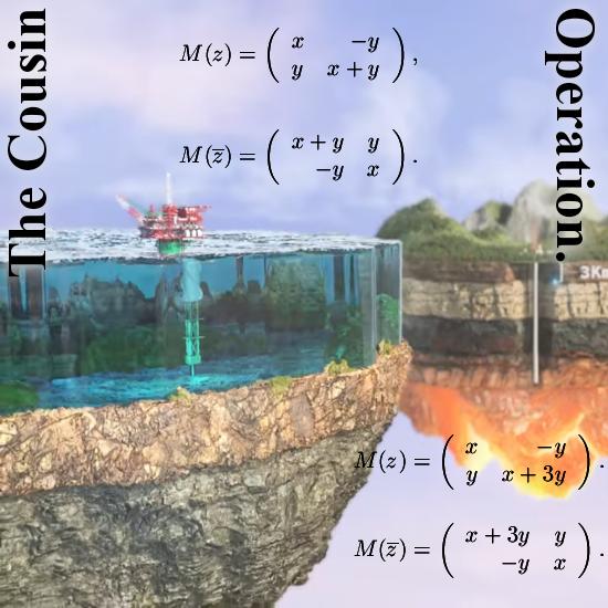
Likely in the year 1991 I had figured out that the conjugate of a 3D complex number could be found in the upper row of it’s matrix representation. As such the matrix representation of a conjugate 3D number was just the transpose of the original matrix representation. Just like we have for ordinary complex numbers from the complex plane. And this transpose detail also showed that if you take the conjugate twice you end where you started from. Math people would say if you do it twice, that is the identity operation. But for the two 2D multiplications we have been looking at in the last couple of months, the method of taking the upper row as a conjugate did not work. I had to do a bit of rethinking and it was not that hard to find a better way of defining the conjugate that worked on all spaces under study since the year 1991. And that method is replace all imaginary units by their inverse. As such we found the conjugate on 2D spaces like the elliptical and hyperbolic complex planes. And the product of a 2D complex number z with it’s conjugate nicely gives the determinant of the matrix representation. And if you look where this determinant equals one, that nicely gives the complex exponentials on these two spaces: an ellipse and a hyperbole. Now when I was writing the last math post (that is two posts back because the previous post was about magnetism) I wondered what the matrix representation of the conjugate was on these two complex planes. It could not be the transpose because the conjugates were not the upper rows. And I was curious what it was, it it’s not the transpose what is it? It had to be something that if you do it twice, you do the identity operation…
All in all in this post the math is not very deep or complicated but you must know how te make the conjugate on say the elliptic complex plane. On this plane the imaginary unit i rules the multiplication by i ^2 = -1 + i. So you must be able to find the inverse of the imaginary unit i in order to craft the conjugate. On top of that you must be able to make a matrix representation of this particular conjugate. If you think you can do that or if you don’t do it yourself you will understand how it all works, this post will be an easy read for you.
It turns out that the matrices of the conjugate are not the transpose where you flip all entries of the matrix into the main diagonal. No, these matrix representation have all their entries mirrored in the center of the matrix or equivalently they have all their entries rotated by 180 degrees. That is the main result of this post.
So that’s why I named it the “Cousin of the transponent” although I have to admit that this is a lousy name just like the physics people have with naming the magnetic properties of the electron as “spin”. That’s just a stupid thing to do and that’s why we still don’t have quantum computers.
Enough intro talk done, the post is five pictures long and each picture is 550×1200 pixels. Have fun reading it.
That was it for this post, one more picture is left to see and that is how I showed it on the other website. Here it is:
Ok, this is really the end of this post. Thanks for your attention and may be see you in another post of this website upon complex numbers.