Monthly Archives: January 2023

A simple example showing the invariance of the determinant (so it returns always a positive number).

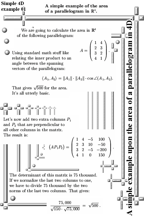
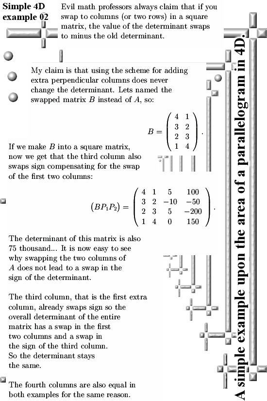
This is one of the details I should have posted last year. So this post is some mustard after the meal. The content is just two pictures long. In it I show you how to calculate the area of a parallelogram in 4D space. After that we swap the two columns and use the same method again. In both cases the area of the parallelogram equal the square root of 500.
If you read stuff from this website you likely have enjoyed some classes in linear algebra, likely you know that if you swap two columns (or two rows) in a square matrix, the determinant changes sign.
But the way we turn a non-square matrix into a square matrix is done in such a way that it has to return a positive (or better: non-negative) number.
In this example you can see that if you swap the two spanning columns of the parallelogram, the first extra column or the third column in our final matrix also chages sign. So the overall determinant of the 4×4 final matrix ‘observes’ a swap in the first two columns and also a swap in the sign of the third column. Hence the determinant does not change sign…

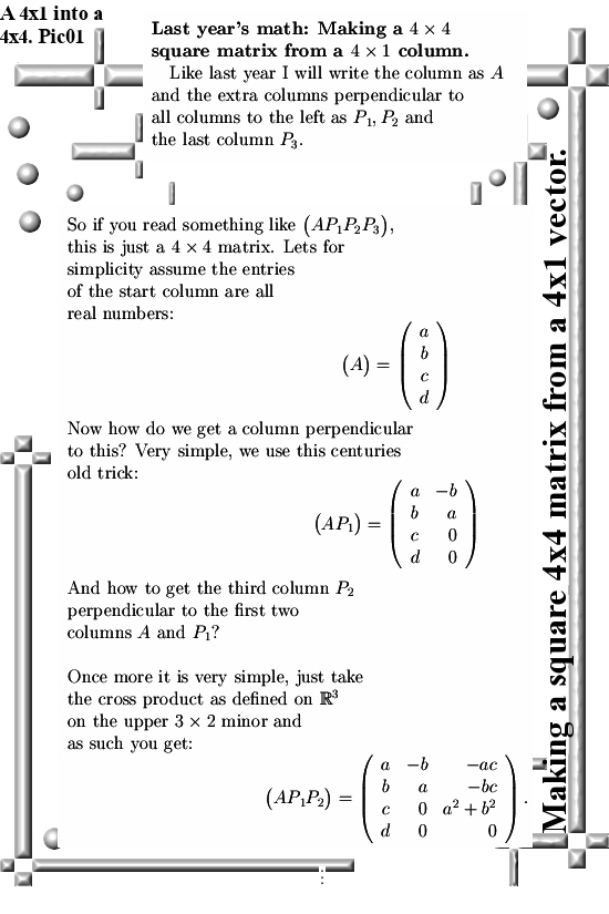
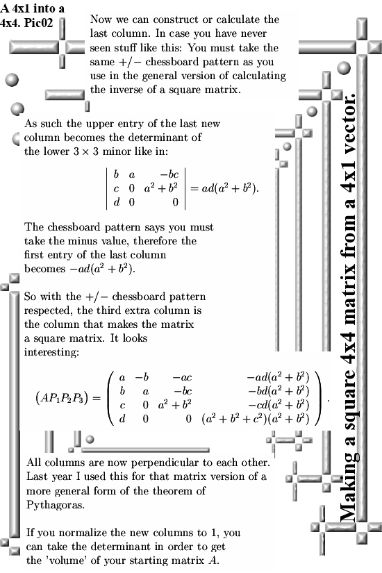
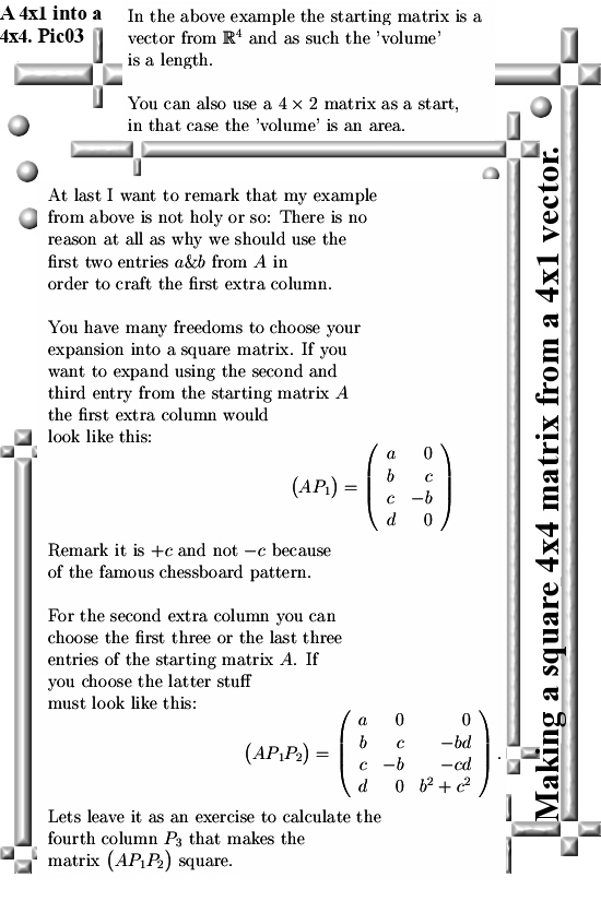
Originally I only needed a few cute looking formulas for use on the other website. That are the two matrices below. But when finished I added some text and as such we have a brand new post for this website.

In this example I did not normalize the extra columns to one so if you want you can play a bit with it and as such observe how their norms are related to the area of the diverse parallograms in here. For example if you calculate the norm of the fourth column, it is the square root of 75,000 while the determinant of the whole 4×4 matrix is 75,000.

As such constructing square matrices like this always leads to the last column having a norm that is the square root of the determinant.
That is a funny property, or not?

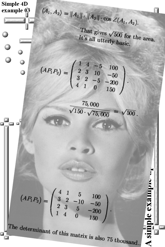
Anyway here are the two pictures, the third picture is an illustration of how it was used on the other website. As usual all pictures have sizes of 550×825.

In the third picture I used an old photo of Brigitte Bardot as a background picture. Now both Brigitte and me we looked a lot more fresh back in the time from before they invented the stone age. Our minds were sharp and our bodies fast while at present day we are just another old sack of skin filled with bones, fat and some muscle. Life is cruel..

Ok, lets end this post now and see you around my dear reader.

Example: How to turn a 4×1 column into a 4×4 square matrix.

Yes I know that two posts back I said that this would be the last time we would do Pythagoras stuff like this. On the other hand I was very unsatisfied with that post (title: That weird root formula). Also I had wanted to post the math below before but I did not have the time.
All in all since I was horribly bad in the post upon that weird root formula about how to make extra columns, may this short post compensates a bit for that.
This post starts with a column of four real numbers, say a, b, c and d. The goal is to keep on adding extra columns such that all columns are perpendicular to each other. Don’t confuse that with an orthogonal matrix, orthogonal matrices also have all their columns perpendicular but the columns are also all of norm one.
For myself I name matrices that have all their columns perpendicular to each other ‘perpendicular matrices’ but this is not a common thing in math communications as far as I know.
I show you two examples here: First I make an extra column based on the a and b entry of our vector. In the second expansion of the same vector I use the middle two entries b and c.
This should serve as examples that make it as transparant as possible how you must use the +/- chessboard pattern that comes with calculations like this.
For understanding this post it comes in very handy if you have done & understand the general way of crafting the inverse of a square matrix. I think most people will see the brilliant +/- chessboard scheme there for the first time in their lives.

I don’t know much about the history of math, but I like it that the +/- chessboard scheme has no human name attached to it like in “Hilbert space”. I guess this chessboard pattern emerged slowly over the cause of a few decades with contributions of many people. So in the end there was nobody to name it too because this big success just had to many fathers.

Another explanation for the lack of a human name to the famous +/- chessboard pattern is that the person who for the first time chrystal clear wrote out the stuff, this person was not an overpaid professional math professors. But say an amateur just like me. Well in those good old times just like now, the overpaid math professors can’t give credit to such an undesireable person of course…
Yet not all is negative when it comes to professional math professors: They are still very good at telling anybody who wants to hear it that: “We tried but we could not find the three dimensional complex numbers”.

After all that human blah blah blah, why not take a look at the three pictures?

Please do that exercise so you can say you understand that +/- chessboard scheme.

That was it for this post.

Two more videos that explain electron spin wrong.

A happy new year by the way, it is now 3 Jan over here so it is not too late to wish you that. So be happy if you can ask a physics professor or teacher as why there is no experimental proof at all that electrons are tiny magnets. And if the answer is not satisfactory, just chop the head of while being happy…;)

But serious, I selected the first video because the guy from the Science Asylum channel gives are very tiny estimated upper bound for the possible size of the electron: 10 to the -18 power meter as diameter.
That is very very small, it is a nano nano meter.

Lets construct a so called ‘toy model’ for imitating in a simple manner how the electron is supposed to be a tiny magnet: Take two pointsize magnetic monopoles, a north and a south one and place them 10 to the power -18 meter apart. Lets name this distance d.
An important feature of such a dipole is that it’s magnetic field declines inversely with the third power of d.

Let me give you an example: Take a line through the north and south pole of our toy electron and go out a distance of say 10d above the north pole. So the distance of our point on that line is 10d to the north pole and 11d to the south pole. The magnetic forces or field strength if you want is now proportional to 1/10^2 and 1/11^2. But north and south pole have opposite workings so we are looking at the difference: 1/10^2 – 1/11^2 and that is something of the order 1/1000.

If the electron diameter is indeed at most this distance d, in that case the two overlapping magnetic fields cancel each other almost out. If all that tiny magnet stuff is true, in that case the electron should be magnetically neutral. In a constant magnetic field that does not vary in space, by definition this tiny magnet electron should be neutral (if it all was true).

Let me show you two screen shots from the video from the Science Asylum. The first simple shows you the claim the electron has at most this size d.

On a nano nano scale this should be magnetically neutral…

A long time ago I estimated the result in next picture too but I always used an electron diameter of 10 to the -16 power, so one hundred time as big as the Asylum guys claims. Anyway there is nothing spinning over there because it must rotate a huge multiple of the speed of light. Now we can honestly say that Albert Einstein did not understand much about electron spin, but we can safely conclude that electron spin is not related to rotation of a spherical charged body the size of d.

One million times the speed of light…

Ok, let me hang in the video where we have once more the implicit claim that magnetism is always a magnetic dipole without one iota of experimental proof for that claim:

In my view the most misleading name is spin, it sets your brain totally wrong.

In the next video you see a guy at work showing that the oxygen in the air you breathe is magnetic. The magnetic properties of oxygen are truly breathtaking because it has to do with a so called ‘non-binding’ electron pair. In chemistry a non-binding electron pair is a pair with the same electron spin. Weirdly enough the physics professors keep their mouth shut: All electron pairs obey the Pauli exclusion principle!
Until it doesn’t like in molecular oxygen.

But I digress, the reason I selected this video can be found at 3.40 minutes into it: The guy ‘explains’ the behavior of the oxygen by stating that the two electrons in the non-binding pair align their magnetic dipole to the applied magnetic field. The problem with this kind of ‘explanation’ is that it does not explain as why the electrons get accelerated. As said above; if electrons are tiny magnetic dipoles, they are basically magnetically neutral. And we are to believe that the oxygen molecules get accelerated by the applied magnetic field because two little electrons ‘align their dipole magnetic moment’. Give me a break: that is crap and the next stuff look much more logical and observable:
Electrons are not magnetic dipoles but magnetic monopoles.

Here is the second video:

The reason for posting this second video is that I often obverve people from physics thinking that the alignment or for that matter the anti-alignment explains the acceleration and forces involved.

After seven years into this stuff I only wonder:

Why do the physics professionals like teachers and professors not see they are telling utter crap? Why are they so fucking stupid all of the time?
End of this post. Once more: A happy new year.