Monthly Archives: August 2018

Part 11 of the 4D complex numbers: The eigenvalues and eigenvectors from the first imaginary unit.

First a short magnetic update:

In reason 66 as why electrons cannot be magnetic dipoles I tried to find a lower bound for the sideway acceleration the electrons have in the simple television experiment.

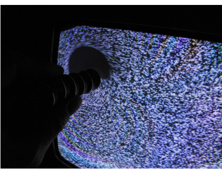
To put it simple: How much sideway acceleration must the electrons have to explain the dark spots on the screen where no electrons land?

The answer is amazing at first sight: about 2.5 times 10^15 m/sec^2.
This acceleration lasts only at most two nano seconds and in the end the minimum sideway speed is about 5000 km/sec so while the acceleration is such a giant number it does not break relativity rules or so…
Here is the link:

16 Aug 2018: Reason 66: Side-way electron acceleration as in the television experiment.
http://kinkytshirts.nl/rootdirectory/just_some_math/monopole_magnetic_stuff03.htm#16Aug2018

You know I took all kinds of assurances that it is only a lower bound on the actual acceleration that takes place. For example I took the maximal sideway distance as only 0.5 cm. Here is a photo that shows a far bigger black spot where no electrons land, so the actual sideway distance if definitely more than 0.5 cm.


__________

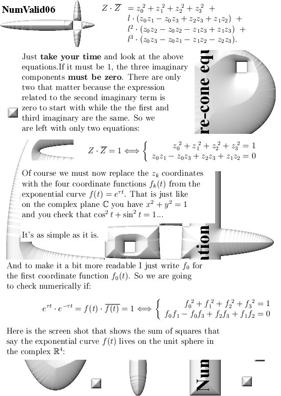
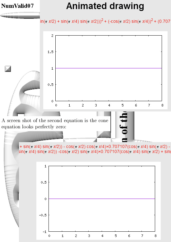
The math part of this post is not extremely thick in the sense you can find the results for yourself with the applet as shown below. Or by pencil & paper find some 4D eigenvalues and the corresponding eigenvectors for yourself.

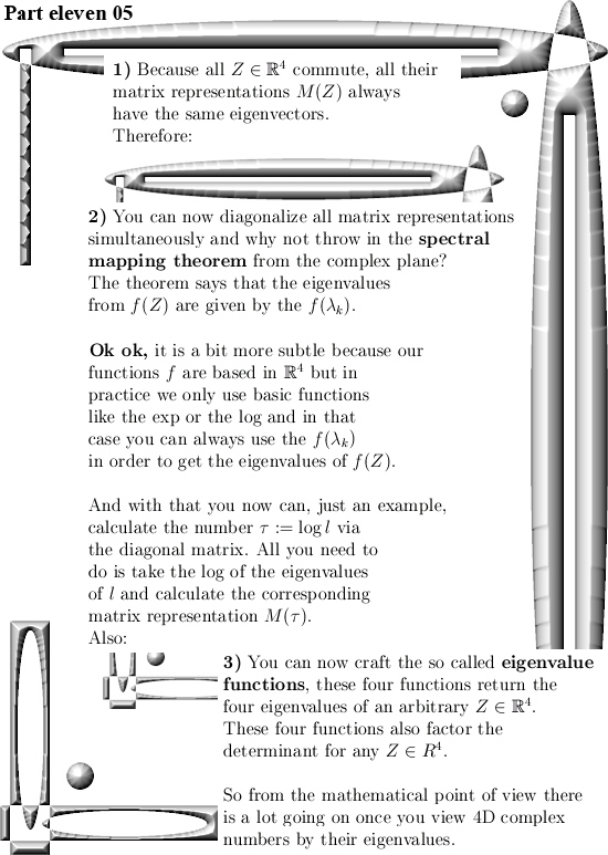
But we need them in order to craft the so called eigenvalue functions and also for the diagonal matrices that come along with all of the matrix representations of the 4D complex numbers Z.

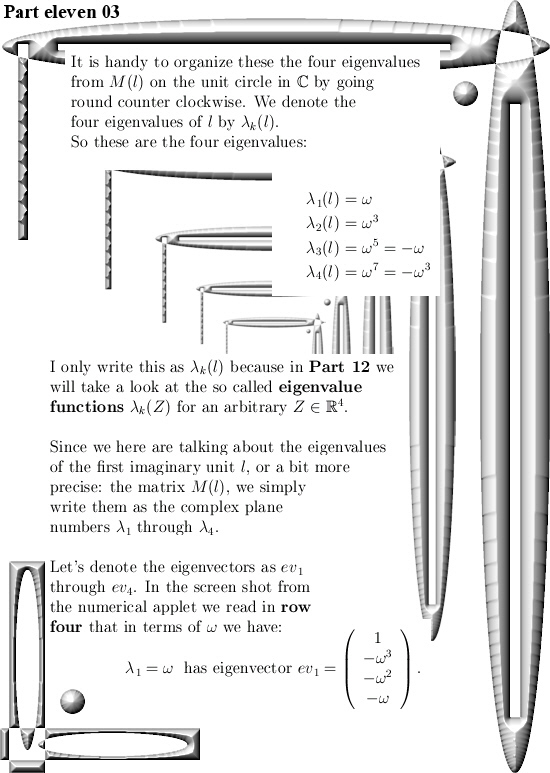
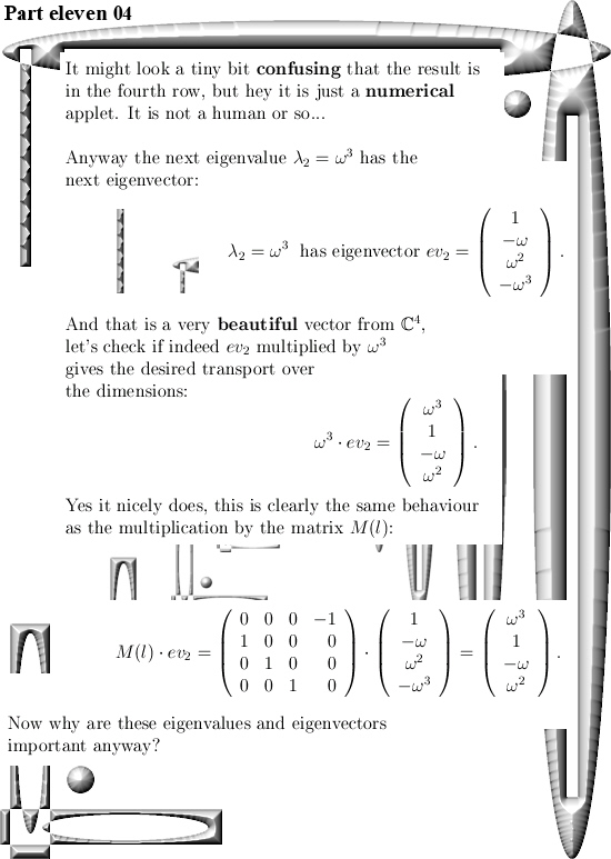
I hope I wrote it down pretty straightforward, this post is five pictures long. And if you like these kind of mathematical little puzzles: Try, given one of the eigenvalues like omega or omega^3, find such an eigenvector for yourself. It is really cute to write them down, multiply them by the eigenvalue and observe with your own eyes that indeed we have all that rotation over the dimensions included that omega^4 = -1 behavior.

This post is five pictures long, it is all rather basic I hope.

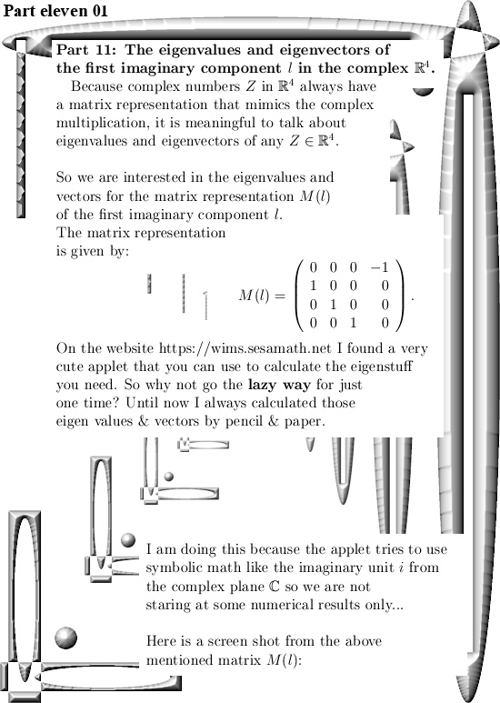
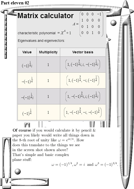
The applet used is from the WIMS server (https://wims.sesamath.net/), look for the Matrix calculator in the section on Online calculators and plotters.

For the time being I think that in Part 12 we will craft the eigenvalue functions for any 4D complex number Z. Ok, that was it for this update.

Part 10 of the 4D basics: The 4D imitators of i rotate everything by 90 degrees.

This is a short and simple update that nicely fits into the series of the basics of 4D complex numbers. It is only 3 pictures long and all we do is multiply a 4D complex number A by one of the imitators of i and after that calculate the inner product between A and A times the imitator of i.

Compare it to the complex plane: Take a 2D complex number z from the complex plane, write it as a vector and also write iz as a vector. Take the inner product and conclude that it is zero so that z and iz are perpendicular to each other.

That’s all we do in the space of 4D complex numbers:

I hope this was basic enough…  See you in the next post.

A few numerical results related to the 4D sphere-cone equations using the four coordinate functions of the 4D exponential curve.

This is Part 9 in the basics to the complex 4D numbers. In this post we will check numerically that the 4D exponential curve has it’s values on the 4D unit sphere intersected with a 4D cone that includes all coordinate axes. In 3D space the sphere-cone equations ensure the solution is 1 dimensional like a curve should be. In 4D space the sphere-cone equations are not enough, there is at least one missing equation and those missing equations can be found in the determinant of a matrix representation M(Z) for a 4D complex number Z.

But we haven’t done any determinant stuff yet (because you also need a factorization of the 4D determinant in four variables and that is not a trivial task). So this post does not contain numerical evidence that the determinant is always one on the entire exponential curve.

If you want to compare this post to the same stuff in the complex plane:
In the complex plane the sphere-cone equation is given by x^2 + y^1 = 1 (that is the unit circle) and if you read this you probably know that f(t) = e^{it} = cos t + i sin t.

You can numerically check this by adding the squares of the sine and cosine for all t in one period and that is all we do in this post. Only it is in 4D space and not in the two dimensional complex plane…

This post is seven pictures long (all of the usual size 550 x 775).

All graphs in this post are made with the applets as found on:

WIMS https://wims.sesamath.net/wims.cgi?lang=en

For the two graphs from above look for ‘animated drawing’ choose the 2D explicit curves option. There you must use the variable x instead of time t.

Here is the stuff you can place in for the sphere equation:

(cos(pi*x/2)*cos(pi*x/4))^2 +
(0.707107*(cos(pi*x/4)*sin(pi*x/2) + sin(pi*x/4)*sin(pi*x/2)))^2 +
(-cos(pi*x/2)*sin(pi*x/4))^2 +
(0.707107*(cos(pi*x/4)*sin(pi*x/2) – sin(pi*x/4)*sin(pi*x/2)))^2

If you just ‘cut & paste’ it should work fine…
That should save you some typo’s along the way

Ok, that is what I had to say on this numerical detail.