Ha, a couple of weeks back I met an old colleague and it was nice to see him. We made a bit of small talk and more or less all of a sudden he said: ‘But you still can always do this’. And he meant getting a PhD in math.
I was a bit surprised he did bring this up, for me that was a station passed long ago. But he made me thinking a bit, why am I not interested in getting a math degree?
And when I thought it out I also had to laugh: Those people cannot go beyond the complex plane for let’s say 250 years. And the only people I know of that have studied complex numbers beyond the complex plane are all non-math people. Furthermore inside math there is that cultural thing that more or less says that if you try to find complex numbers beyond the complex plane, you must have a ‘mental thing’ because have you never heard of the 2-4-8 theorem?
Beside this, if I tried it in the years 1990 and 1991 with very simple: Here this is how the 3D Cauchy Riemann equations look… And you look them in the eyes, but there is nothing happening behind those eyes or in the brain of that particular math professor. Why the hell should I return and under the perfect guidance of such a person get a PhD?
I am not a masochist. If complex numbers beyond the complex plane are ignored, why try to change this? After all this is a free world and most societies run best when people can do what they are good at. Apparently math like I make simply falls off the radar screen, I do not have much problems with that.
___________
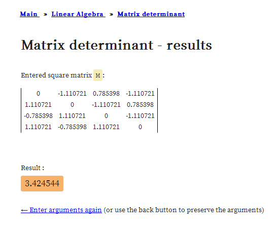
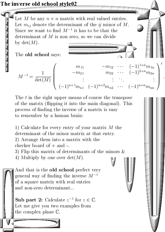
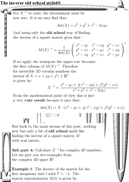
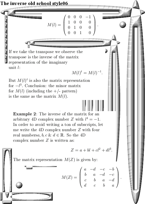
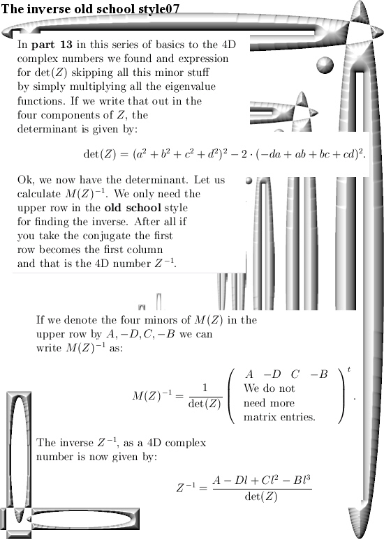
After having said that, this update Part 17 in the basics to the 4D complex numbers is as boring as possible. Just finding the inverse of a matrix just like in linear algebra with the method of minor matrices.
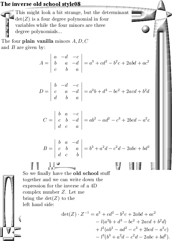
Believe me it is boring as hell. And after all that boring stuff only one small glimmer of light via crafting a very simple factorization of the determinant inside the 4D complex numbers. So that is very different from the previous factorization where we multiplied the four eigenvalue functions. From the math point it is a shallow result because it is so easy to find but when before your very own eyes you see the determinant arising from those calculations, it is just beautiful. And may be we should be striving a tiny bit more upon mathematical beauty…
This post is nine pictures long in the usual size of 550×775 pixels.

As an antidote against so much polynomials like det(Z), with 2 dimensions like a flatscreen television, you can do a lot of fun too. The antidote is a video from the standupmaths guy, it is very funny and has the title ‘Infinite DVD unboxing video: Festival of the Spoken Nerd’. Here is the vid:
End of this update, see you around.
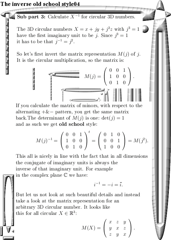
Ok ok, a few days later I decided to write a small appendix to this post and in order too keep it simple let’s calculate the determinant of the 3D circular numbers. I have to admit this is shallow math but despite being shallow it gives a crazy way to calculate the determinant of a 3D circular number…
So a small appendix, here it is:
And now you are really at the end of this post.
In the next post let’s calculate the inverse of the 4D complex tau number. After all a few months back I gave you the new Cauchy integral representation and I only showed that the determinant of tau was nonzero.
But the fact that the Cauchy integral representation is so easy to craft on the 4D complex numbers arises from the fact the inverse of tau exists in the first place. In 3D the number tau is not invertible, and Cauchy integral representations are much more harder to find.
Ok, drink a green tea or pop up a fresh pint, till updates.