Recently I am working on part 20 to the basics of the 4D complex numbers. Ok ok if you need 20 parts to explain ‘the basics’ how basic is it you can ask yourself.
You can argue long and short on this: are fresh Cauchy integral formula’s really ‘basic stuff’? I don’t know how a democratic vote among professional math professors would fall down.
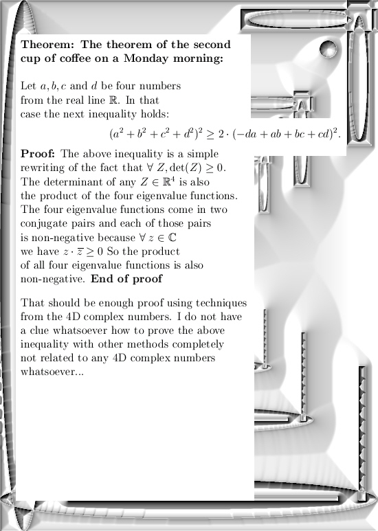
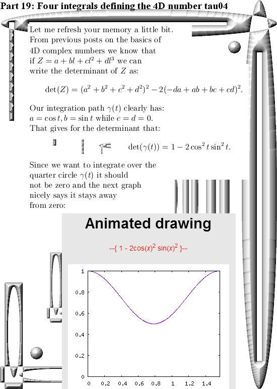
Anyway, an important property of the determinant of 4D complex numbers is the fact that the determinant is always non-negavite. At least it is zero and at those points in space we have found a non-invertible number.
In part 20 on the basics to 4D complex numbers we will look when the eigenvalues of 4D complex numbers vanish; at those points the stuff is non-invertible & that is what we will be hunting on part 20.
In the next picture you see a difficult to understand inequality & the teaser question is:
Can you prove this inequality via math methods that do not use 4D complex number theory at all?
If so, you should definitely pop up a second pint of perfect beer on a late Friday evening.
Ok, that was it. Till updates in part 20 where we try to find all non-invertible 4D complex numbers in a not too difficult way.
Somewhere last year I just looked some nice video from the Mathologer about the theorem of Pythagoras. And since I myself have found a proof for the general theorem of Pythagoras in higher dimensions, I was puzzled about what the so called ‘inverse theorem of Pythagoras’ actually was.
Could I do that too in my general proof? And the answer was yes, but when I wrote that old proof of the general theorem of Pythagoras it was just a technical blip not worthwhile mentioning because it was a simple consequence of how those normal vectors work.
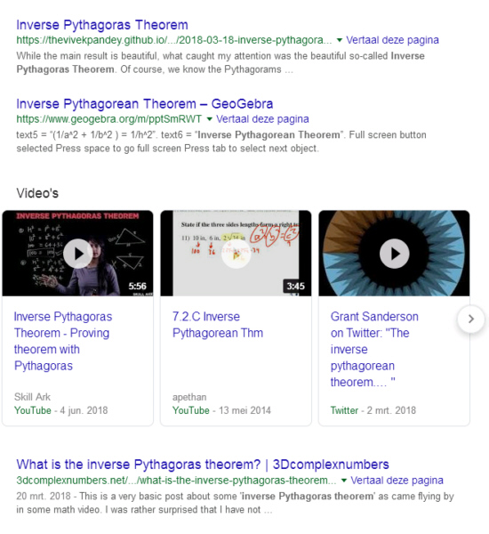
Anyway to make a long story short, a few days back I likely had nothing better to do and for some reason I did an internet search for ‘the inverse theorem of Pythagoras’. All I wanted to do is read a bit more about that from other people.
To my surprise my own writing popped up as search result number 3, that was weird because I wanted to read stuff written by other people… Here is a screenshot of the answers as given by the Google search machine:
Ok ok, not bad at search result number 3.
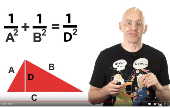
Now why bring this up? Well originally I forgot to post to the video that started my thinking in the first place. It is from the Mathologer and here at 16.00 minutes into his video is where my mind started to drift off:
The video from the Mathologer is here (title Visualizing Pythagoras: ultimate proofs and crazy contortions):
It is a very good video, my compliments.
After so much advertisements for the Mathologer, just a tiny advertisement for what I wrote on the subject of the inverse theorem of Pythagoras on March 20 in the year 2018:
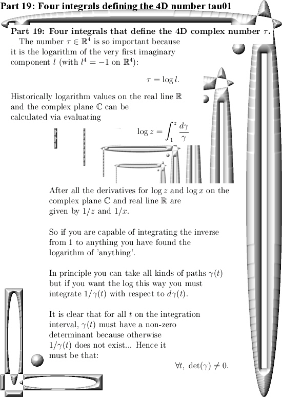
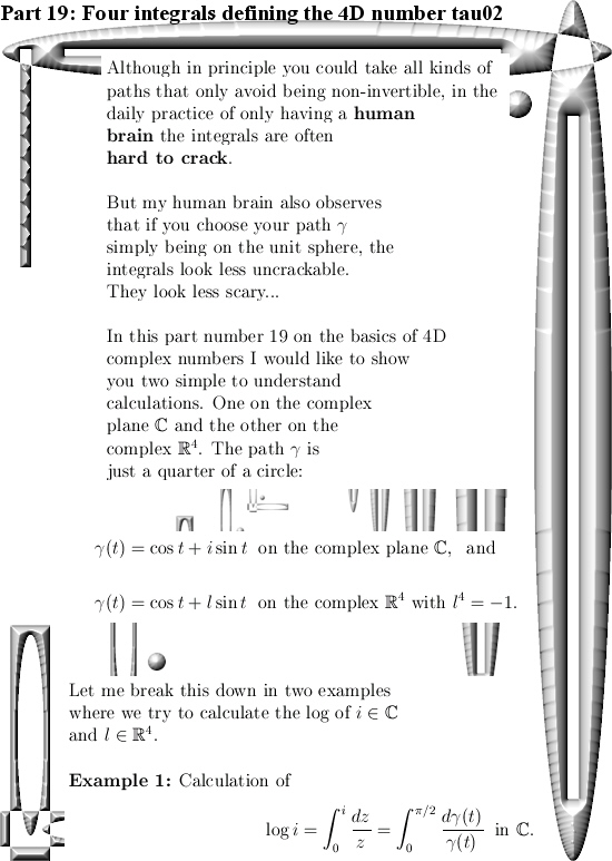
It is a bit late but a happy new year anyway! In this post we will do a classic from the complex plane: calculation of the log of the first imaginary unit.
On the complex plane this is log i and on the complex 4D space this is log l .
Because this number is so important I have given it a separate name a long long time ago: These are the numbers tau in the diverse dimensions. In the complex plane it has no special name and it simply is i times pi/2.
On the real line it is pretty standard to define the log functions as the integral of the inverse 1/x. After all the derivative of log x on the real line is 1/x and as such you simply define the log to be the integral of the derivative…
On the complex plane you can do the same but depending of how your path goes around zero you can get different answers. Also in the complex plane (and other higher dimensional number systems) the log is ‘multi valued’. That is a reflection of the fact we can find exponential periodic functions also known as the exponential circles and curves.
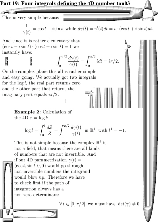
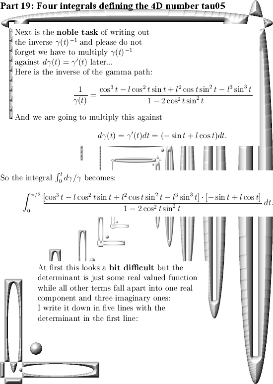
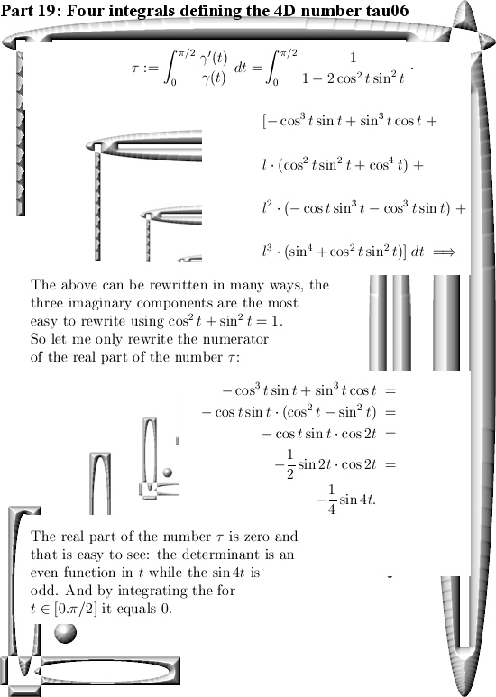
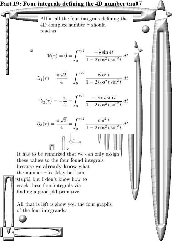
The integrals in this part number 19 on the basics of 4D complex numbers are very hard to crack. I know of no way to find primitives and to crack them that way. May be that is possible, may be it is not, I just do not know. But because I developed the method of matrix diagonals for finding expressions for the value of those difficult looking integrals, more or less in an implicit manner we give the right valuations to those four integrals.
With the word ‘implicit’ I simply mean we skip the whole thing of caculating the number tau via matrix diagonalization. We only calculate what those integrals actually are in terms of a half circle with coordinates cos t and sin t.
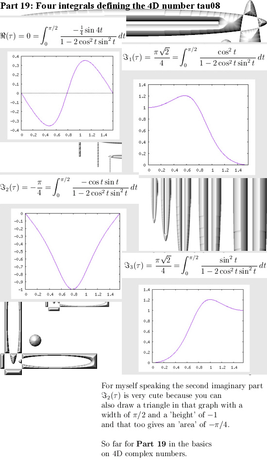
This post is 8 pictures long in the usual size of 550 by 775 pixels (I had to enlarge the latest picture a little bit). I hope it is not loaded with typo’s any more and you have a more or less clean mathematical experience:
There is more than one candidate; the possible explanation of those solar loops via the rotating plasma under it is indeed very very nice.
But it is very hard to find experimental evidence for that, how to check that on the sun where there is one of those solar loops, the solar plasma underneath it is rotating?
So my choice for this year most beautiful insight is how those magnetic domains in materials like iron actually work. If my thinking on electrons as magnetic monopoles is correct, you could view those magnetic domains as surplusses of either north-pole electrons or south-pole charged electrons.
This should be much more easy to verify experimentally. After all there is still plenty of magnetic tape around and the best way of checking if magnetic domains are suplusses of one of the two magnetic charges is much more handy if you have a flat surface like magnetic tape.
Furthermore at present day it should be possible to measure very small magnetic charges. After all in most computers there still are spinning hard disks that use magnetism as the basic information storage.
Anyway to make a long story short: If in a flat material like magnetic tape you can go around a magnetic domain with a tiny compass, all of the time the tiny compass should point towards that magnetic domain with the same side of the compass needle.
So it should always point with the north-pole of the compass needle or the south-pole of the compass needle. Remark that according to standard physics theory going around a magnetic domain should always give different readings with a tiny compass needle…
Also in that line of thinking, the domain walls shoud have surplusses of electron pairs that all are spinning around to compensate or neutralize the magnetic forces they feel. An important clue to that lies in the fact you cannot really move or transport domain walls in a wire as the engeneers of IBM tried with making their nano wire racetrack memory.
This year we heard more or less nothing from IBM with progress into the concept of nano wire racetrack memory. Yeah yeah, the price of not understanding electron spin is huge, if we could have fast computer memory that uses very little energy that would be great…
This year I also gave up on my fantasies of trying to make an official publication in some physics yournal. I don’t think such a publication will ever pass the peer review that those scientific yournals use. Those peer review people just want the electron is a magnetic dipole and that’s it. So I did not try that this year nor will I try next year.
Not that I am aginst peer review. Suppose there would be zero peer review and think for example medical scientific publications. They would be filled with all kind of weird benefits that homeopathy therapy has, or the healing of your chakra’s with mineral chrystals… Of course we cannot have that. As such there must always be the so called peer review…
Ok, the word count counter says 500+ words written so I have to stop writing.
Here is the link to what I self more or less consider as the best improving insight on my behalf on the behavior of all things magnetic. It is from 7 July this year:
This is the shortest post ever written on this website.
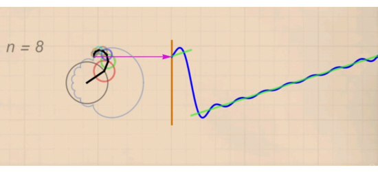
I found one of those video’s where the Fourier series is explained as the summation of a bunch of circles. Likely when you visit a website like this one, you already know how to craft a Fourier series of some real valued function on a finite domain.
You can enjoy a perfect visualization of that in the video below:
Only one small screen shot from the video:
Oh oh, the word count counter says 80+ words. Let me stop typing silly words because that would destroy my goal of the ‘shortest post ever’. Till updates.
It is the shortest day of the year today and weirdly enough I like this kind of wether better compared to the extreme heat of last summer. Normally I dislike those long dark days but after so much heat for so long I just don’t mind the darkness and the tiny amounts of cold.
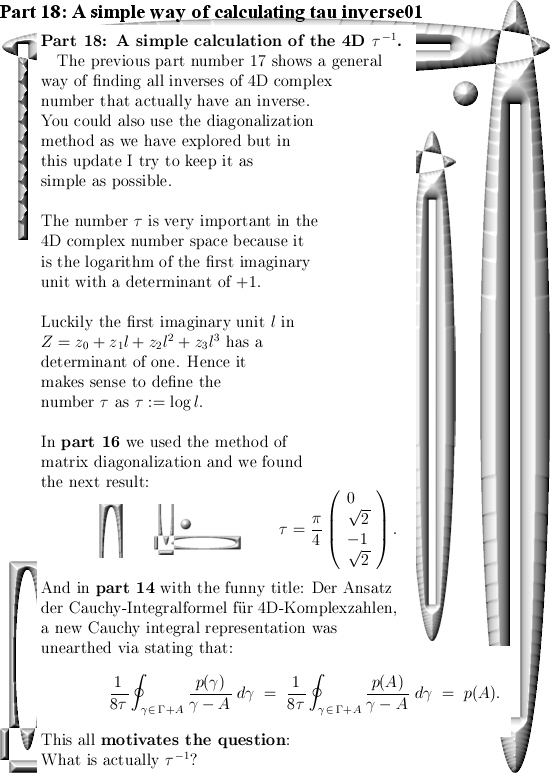
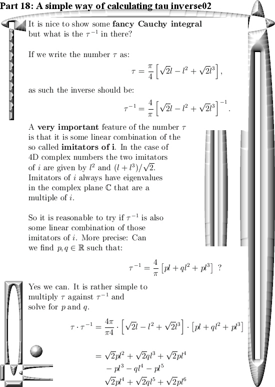
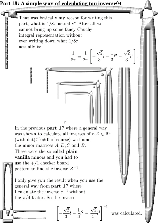
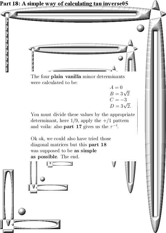
In the previous post we found a general way of finding all inverses possible in the space of the 4D complex numbers. Furthermore in the post with the new Cauchy integral representation we had to make heavy use of 1/8tau and as such it is finally time to look at what the inverse of tau actually is.
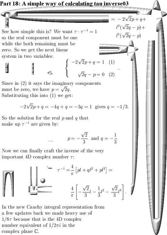
I found a very simple way of calculating the inverse of the number tau. It boils down to solving a system of two linear equations in two variables. As far as I know reality, most math professionals can actually do this. Ok ok, for the calculation to be that simple you first must assume that the inverse ‘looks like’ the number tau in the sense it has no real component and it is just like tau a linear combination of those so called ‘imitators of i‘.
This is a short post, only five pictures long. I started the 4D complex number stuff somewhere in April of this year so it is only 8 month down the timeline that we look at the 4D complex numbers. It is interesting to compare the behavior of the average math professor to back in the time to Hamilton who found the 4D quaternions.
Hamilton became sir Hamilton rather soon (although I do not know why he became a noble man) and what do I get? Only silence year in year out. You see the difference between present day and past centuries is the highly inflated ego of the present day university professors. Being humble is not something they are good at…
After having said that, here are the five pictures:
All in all I have begun linking the 4D complex numbers more and more in the last 8 months. On details the 4D complex numbers are very different compared to 3D and say 5D complex numbers but there are always reasons for that. For example the number tau has an inverse in the space of 4D complex numbers but this is not the case in 3 or 5D complex numbers space.
Well, have a nice Christmas & likely see you in the next year 2019.
Ha, a couple of weeks back I met an old colleague and it was nice to see him. We made a bit of small talk and more or less all of a sudden he said: ‘But you still can always do this’. And he meant getting a PhD in math.
I was a bit surprised he did bring this up, for me that was a station passed long ago. But he made me thinking a bit, why am I not interested in getting a math degree?
And when I thought it out I also had to laugh: Those people cannot go beyond the complex plane for let’s say 250 years. And the only people I know of that have studied complex numbers beyond the complex plane are all non-math people. Furthermore inside math there is that cultural thing that more or less says that if you try to find complex numbers beyond the complex plane, you must have a ‘mental thing’ because have you never heard of the 2-4-8 theorem?
Beside this, if I tried it in the years 1990 and 1991 with very simple: Here this is how the 3D Cauchy Riemann equations look… And you look them in the eyes, but there is nothing happening behind those eyes or in the brain of that particular math professor. Why the hell should I return and under the perfect guidance of such a person get a PhD?
I am not a masochist. If complex numbers beyond the complex plane are ignored, why try to change this? After all this is a free world and most societies run best when people can do what they are good at. Apparently math like I make simply falls off the radar screen, I do not have much problems with that.
___________
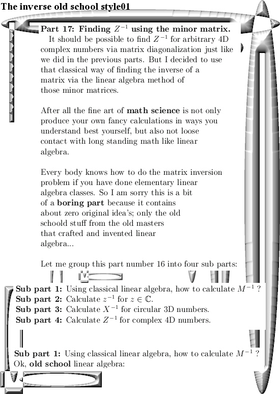
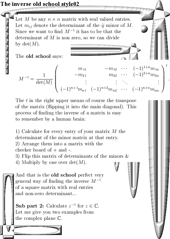
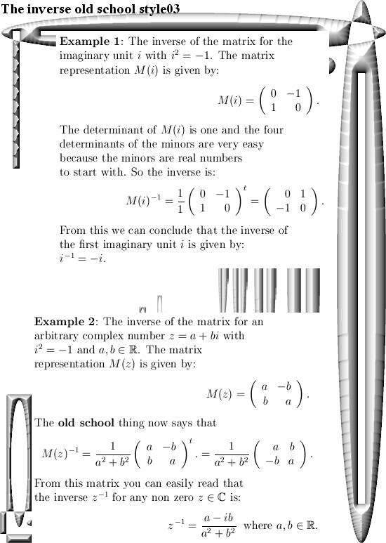
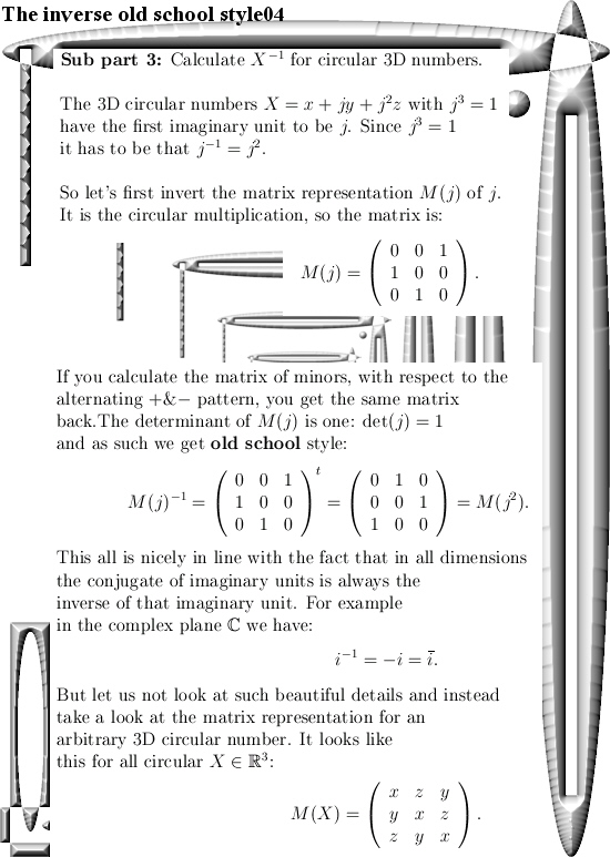
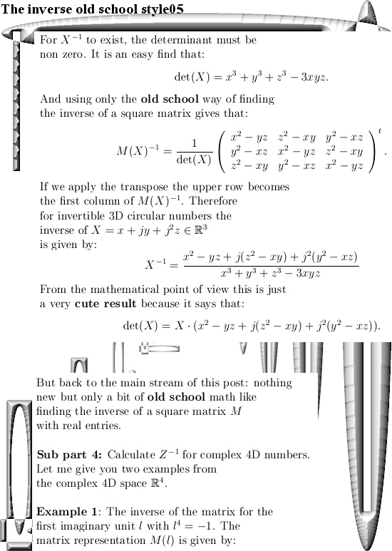
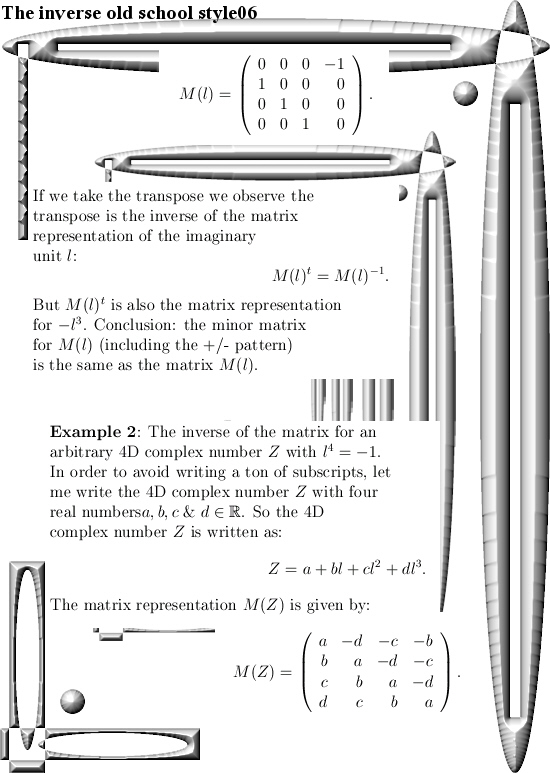
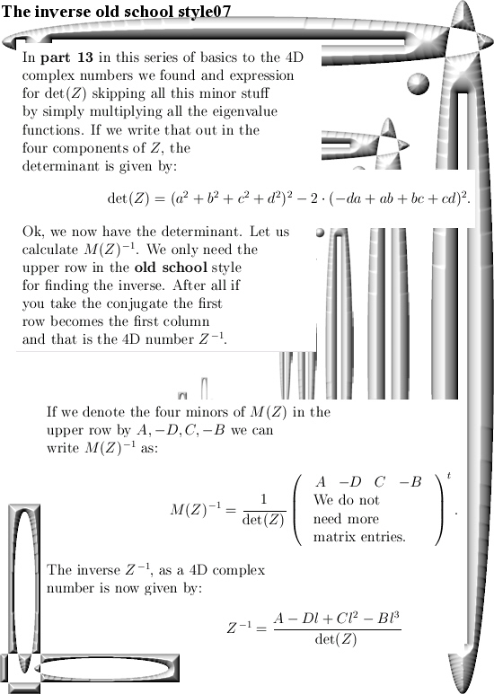
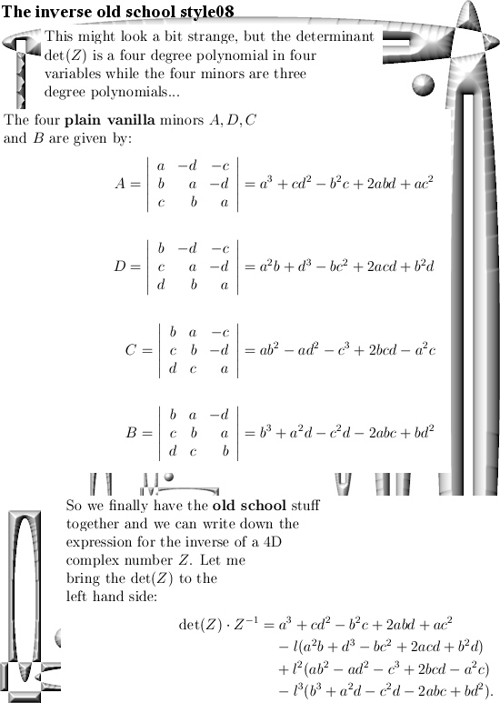
After having said that, this update Part 17 in the basics to the 4D complex numbers is as boring as possible. Just finding the inverse of a matrix just like in linear algebra with the method of minor matrices.
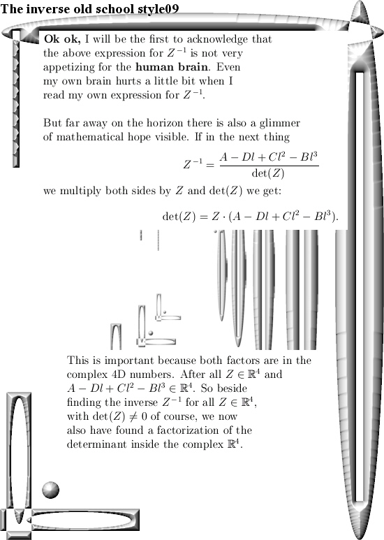
Believe me it is boring as hell. And after all that boring stuff only one small glimmer of light via crafting a very simple factorization of the determinant inside the 4D complex numbers. So that is very different from the previous factorization where we multiplied the four eigenvalue functions. From the math point it is a shallow result because it is so easy to find but when before your very own eyes you see the determinant arising from those calculations, it is just beautiful. And may be we should be striving a tiny bit more upon mathematical beauty…
This post is nine pictures long in the usual size of 550×775 pixels.
As an antidote against so much polynomials like det(Z), with 2 dimensions like a flatscreen television, you can do a lot of fun too. The antidote is a video from the standupmaths guy, it is very funny and has the title ‘Infinite DVD unboxing video: Festival of the Spoken Nerd’. Here is the vid:
End of this update, see you around.
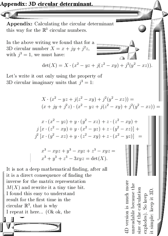
Ok ok, a few days later I decided to write a small appendix to this post and in order too keep it simple let’s calculate the determinant of the 3D circular numbers. I have to admit this is shallow math but despite being shallow it gives a crazy way to calculate the determinant of a 3D circular number…
So a small appendix, here it is:
And now you are really at the end of this post.
In the next post let’s calculate the inverse of the 4D complex tau number. After all a few months back I gave you the new Cauchy integral representation and I only showed that the determinant of tau was nonzero.
But the fact that the Cauchy integral representation is so easy to craft on the 4D complex numbers arises from the fact the inverse of tau exists in the first place. In 3D the number tau is not invertible, and Cauchy integral representations are much more harder to find.
Ok, drink a green tea or pop up a fresh pint, till updates.
There is a Youtube channel named the science asylum. It is run by a guy that makes your head tired but for a few minutes it is often nice to watch. In the next video he tries to explain magnetism, both electro-magnetism and permanent magnets.
Here is the video:
The video guy tries to explain permanent magnets via the concept of angular momentum. As far as I know physics now this is indeed the way it has historically evolved. Now a lot of physics folks think that the unpaired electrons somehow go around the nucleus and as such create a magnetic dipole moment, other place more emphasis on electrons being the basic dipole magnets and if they align all conditions for possible permanent magnets are there. Of course beside electrons also the so called magnetic domains need to align and the official version is that this is more or less the way some materials like iron can be turned into permanent magnets.
In my view there is a long list of problems that come with that. For example the Curie temperature, above the Curie temperature the permanent magnet looses it’s magnetism completely.
If you view electrons as magnetic monopoles, stuff like the Curie temperature become a lot more logical: above the Curie temperature it has to be that the metal is so hot it starts to loose it’s unpaired electrons.
In my view, when permanent magnets are manufactured it is the applied external magnetic field and the slow slow cooling down from above the Curie temperature that ensures the magnet becomes ‘permanent’.
There should be a simple experimental proof for that but although for years I tried to find it, until now I still haven’t found it. But in our global industrie a lof of permanent magnets are made every day and the experimental proof for my view on electron spin simply says the next:
If during the cooling down a NS external magnetic field is applied, the permanent magnet will come out as a SN magnet.
With SN I simply mean that the magnetic south pole is on the left while the magnetic north pole is on the right. So the macroscopic object known as the permanent magnet will always be anti-aligned with the magnetic field that is applied during the fabrication of the permanent magnet.
I still haven’t found it after all these years, but if it comes out that permanent magnets have the same orientation as the applied external magnetic field during fabrication, I can trash my theory of magnetic charges and finally go on with my life…
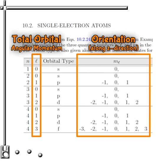
But there are plenty of problems more with the standard model version of electrons being magnetic dipoles. Here is a screen shot from 4.35 minutes into the video from the crazy asylum guy and it contains so called quantum numbers.
The title in the picture might look a bit confusing because the only single-electron atom in the universe is the hydrogen atom. Likely the author means the number of unpaired electrons in some atom.
You observe two quantum numbers that are holy inside quantum mechanics:
The so called ‘Total orbital angular momentum’ number l and something weird because it is only along the z-axis direction m_l.
In my view, if electrons carry magnetic charge and are not magnetic dipoles and for example it has 3 unpaired electrons, total magnetic charge runs from -3 to +3.
And that is precisely what the m subscript l number does…
So I still have to find the very first fault in my simple idea that electrons just carry one of the two possible magnetic charges.
In this post I skipped the fourth quantum number: total spin. That is also a quantum number thing so is it a vector (a magnetic dipole) or a magnetic charge (a magnetic monopole)?
Ok, let’s leave it with that. Have a nice set of quantum numbers or try to get one.
Added on 26 Nov:
May be looking at chaotic guys makes me chaotic too, but reading back what I wrote yesterday I think it is better to explain the ‘anti alignment’ a bit more because I explained it far too confusing I just guess.
I made a schematic sketch of it, you see two coils that make a long lasting constant magnetic field and in that field a hot piece of iron is slowly cooling down. An important feature of iron is that the four unpaired electrons are in the inner shells, this is a consequence of the so called aufbau principle.
Here is the sketch:
So my basic idea of manufacturing permanent magnets is the fact that during the long cool down the unpaired electrons can settle in those inner shells inside the electron could of the iron atoms.
Furthermore it has to be that the chrystal structure metals like iron make is such that the individual iron atoms cannot rotate. It is fixed in place. And with the unpaired magnetic charge carrying electrons in place after the long cool down, that is why your permanent magnet is more or less permanent:
Small surplusses of south charged electrons should be at the left & vice versa a bit more north magnetic charge at the right as sketched above.
This all sounds very simple but we also have those magnetic domains in metals like iron, those magnetic domains are just small surplusses of either one of the two magnetic charges. This blurs the simplicity a bit but it perfectly explains as why unmagnetized iron gets attracted to magnets anyway: the dynamics of the magnetic domain changes under the influence of the outside permanent magnet…
At last I want to remark that if the idea of permanent magnetism would solely based on dipole electron spin that aligns, in that case strong permanent magnets should change the permanent magnetism of weakly magnetized iron. The strong magnets would simply eat up the electrons of the weak permanent magnet.
That just does not happen. Last spring I made a small toungue in cheek ‘experiment’ with that where I placed my stack of most strong neodymium magnets against two of my most weak magnets. It was all fixed in place over 24 hours, but after all that time my two most weak permanent magnets exposed the same behaviour as before.
So no electron was flipped and for me that was one more reason to say farewell to the idea of electrons being magnetic monopoles.
Here is a link to that very simple toungue in cheek experiment, I hope it is so simple that physics professors will vomit on that…
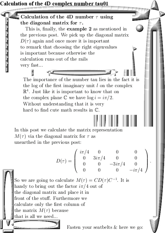
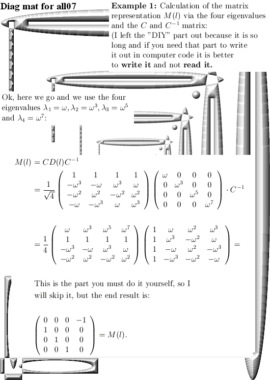
In the begin of this series on basic and elementary calculations you can do with 4D complex numbers we already found what the number tau is. We used stuff like the pull back map… But you can do it also with the method from the previous post about how to find the matrix representation for any 4D complex number Z given the eigenvalues.
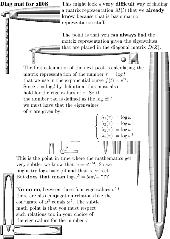
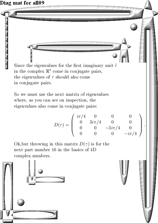
Finding the correct eigenvalues for tau is rather subtle, you must respect the behavior of the logarithm function in higher dimensions. It is not as easy as on the real line where you simply have log ab = log a + log b for positive reals a and b.
But let me keep this post short and stop all the blah blah.
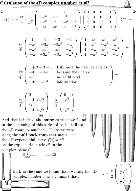
Just two nice pictures is all to do the calculation of the 4D complex number tau:
(Oops, two days later I repaired a silly typo where I did forget one minus sign. It was just a dumb typo that likely did not lead to much confusion. So I will not take it in the ‘Corrections’ categorie on this website that I use for more or less more significant repairs…)
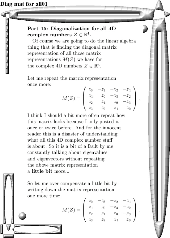
This website is now about 3 years old, the first post was on 14 Nov 2015 and today I hang in with post number 100. That is a nice round number and this post is part 15 in the series known as the Basics for 4D complex numbers.
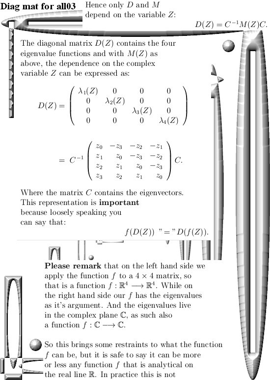
We are going to diagonalize all those matrix representations M(Z) we have for all 4D complex numbers Z. As a reader you are supposed to know what diagonalization of a matrix actually is, that is in most linear algebra courses so it is widely spread knowledge in the population.
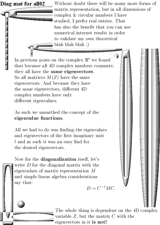
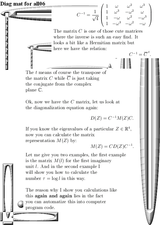
Now at the end of this nine pictures long post you can find how you can calculate the matrix representation for M(l) where l is the first imaginary unit in the 4D complex number system. And I understand that people will ask full of bewilderment, why do this in such a difficult way? That is a good question, but look a bit of the first parts where I gave some examples about how to calculate the number tau that was defined as log l. And one way of doing that was using the pull back map but with matrix diagonalization you have a general method that works in all dimensions.
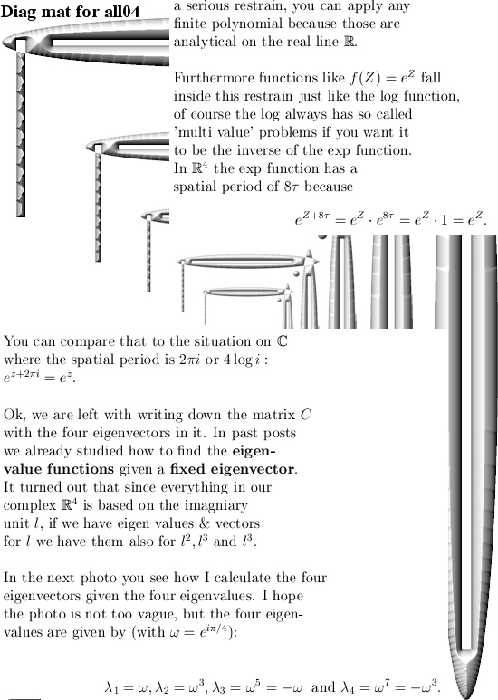
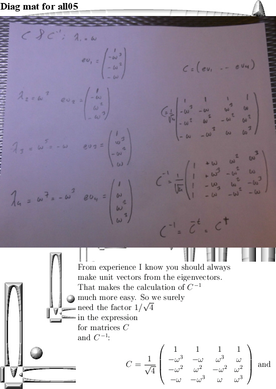
Beside that this is an all inclusive approach when it comes to the dimension, in practice you can rely on internet applets that use commonly known linear algebra. Now if you are a computer programmer you can automate the process of diagonalization of a matrix. I am very bad in writing computer programs, but if you can write code in an environment where you can do symbolic calculus in your code, it would be handy if that is on such a level you can use the so called roots of unity from the complex plane. After all the eigenvalues you encounter in the 4D complex number system are always based on these roots of unity and the eigenvectors are too…
This post number 100 is 9 pictures long, as usual picture size is 550 x 775 pixels.
In the next post number 101 we will use this method to calculate the matrix representation of the number tau (that is the log of the first imaginary unit l).
Ok, here are the pictures:
That´s it, in the next post we go further with the number tau and from the eigenvalues of tau calculate the matrix representation. So see you around.