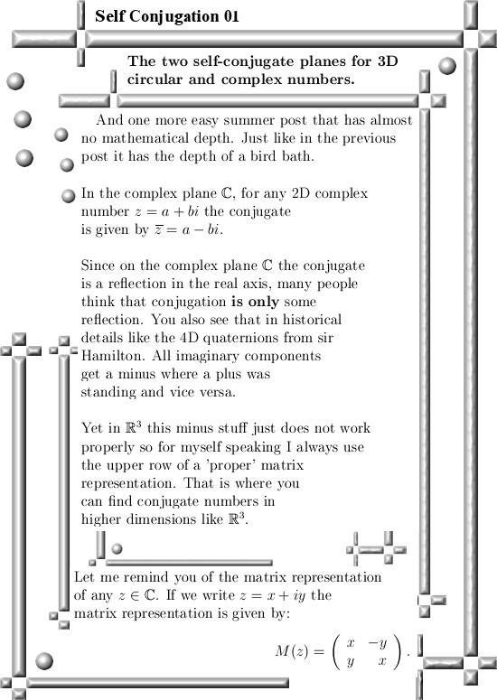
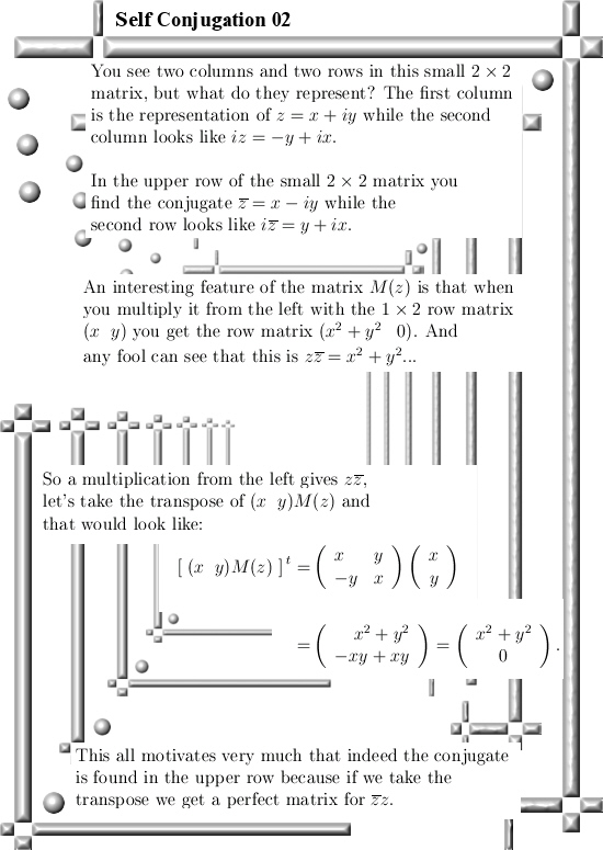
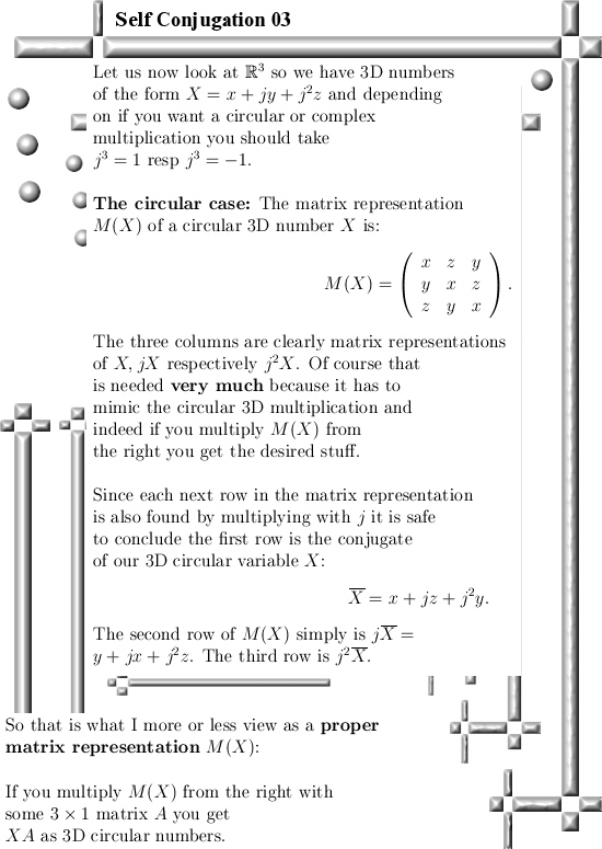
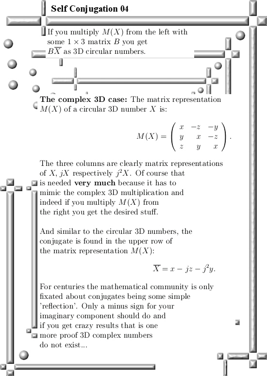
This is another lightweight easy going summer update. It is about matrix representations and how to find the conjugate of a 3D complex or circular number. I use the case of the complex plane of 2D conplex numbers to show that conjugation is not some silly reflection just always but rather simple will always be the upper row of a proper matrix representation. As a matter of fact it is so easy to understand that even the biggest idiots on this planet could understand it if they wanted. Of course math professors don’t want to understand 3D numbers so also this new school year nothing will happen on that front…
Did you know that math professors study the periodic system? Yes they do, anyway in my home country the Netherlands they do because every year they get a pay rise and that pay rise is called a periodic. And as such they study the periodic system deep and hard…
I classified this post only under the categories ‘3D complex numbers’ and ‘matrix representations’ and left all stuff related to exponential circles out. Yet the exponential circle stuff is interesting; after reading this post try to find out if the numbers alpha (the midpoint of the exponential circles) are symmetrix (yes). And the two numbers tau (the log of the first imaginary unit on the circular and complex 3D space) are anti-symmetrix (yes).
This post is just over 7 pictures long. As the background picture I used the one I crafted for the general theorem of Pythagoras. (Never read that one? Use the search funtion for this website please!) All pictures are of the usual size namely 550×775 pixels.
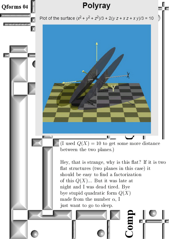
Ok, that was it for this update. Although it is so very simple (for years I did not want to write of just two simple planes that contain all the self-conjugate numbers) but why make it always so difficult? Come on it is summer time and in the summer almost all things are more important than math. For example goalkeeper cat is far more important compared to those stupid 3D numbers. So finally I repost a video about a cat and that makes me very similar to about 3 billion other people.
Till updates & thanks for your attention.