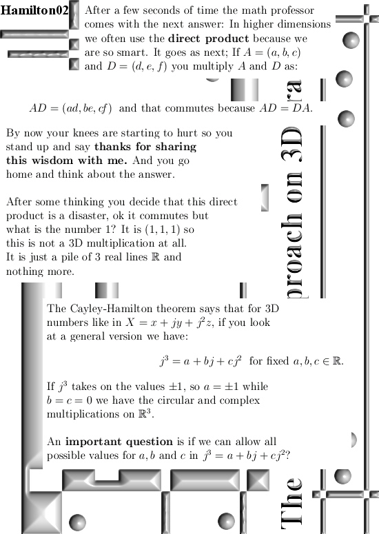
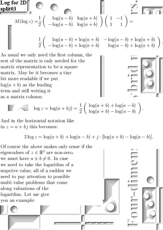
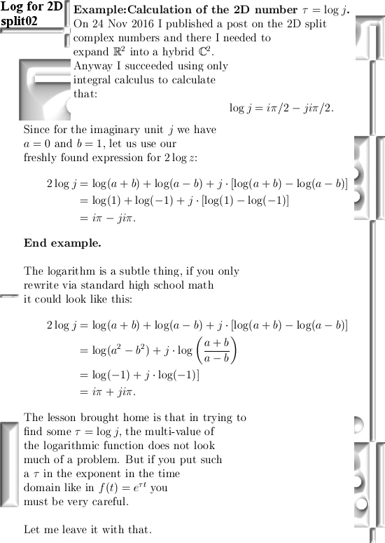
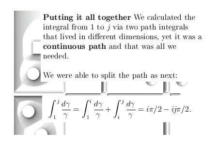
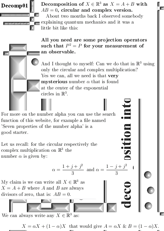
I got the idea for this post already a couple of years back but I shelved it because I would like to have some application for it. But I still haven’t found a killer application yet anyway I decided to write this rather simple post about the projections you get when you multiply any 3D complex and circular numbers with the number alpha. If you need a refreshment on the importance of the number alpha (or what it actually is) please use the search function of this website and search for ‘Seven properties of the number alpha’.
Now two months back I observed some guy in a video explaining the math you need for quantum physics (yes I have a very boring life) and he was explaining you also need projectors P such that P^2 = P meaning that if P is some measuring operator, if you measure it twice you get the same result. And ha, now I write this post down I realize I did not prove that for both operators in the pictures below so that is something you can do for yourself if you want that.
Basically it goes as next: Pick any 3D number X, circular or complex, and multiply it by the number alpha. The result is a number on the main axis of non-invertible numbers (and as such an entire 2D plane gets projected on each of the main axis non invertible numbers). The other operator is (1 – alpha) and if you multiply any 3D number X by that, it gets projected on the plane of non-invertible numbers (and as such a line gets projected on a point of that plane).
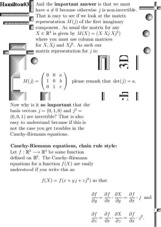
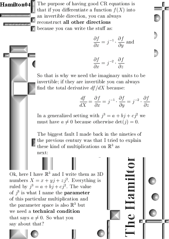
All in all it is very basic, but ha ha ha I am doing this stuff now for years on a row and may be for the average reader it is all not so basic. This post is easier to grasp if you understand the shape of the non-invertible numbers: it is a plane and perpendicular on that plane the main axis and both the plane and main axis go through zero. In this post I skipped all things eigenvalue, but in 3D space we have 3 eigenvalues per capita number so unlike in 4D space we cannot have eigenvalue pairs only. In 3D space it has to be different and that explains more or less the shape of the non-invertible numbers.
This post is five pictures long, as usual all 550×775 pixels and I really hope it is not that hardcore this time.
Before we split, on the other website I posted reason number 73 as why electrons cannot be magnetic dipoles. I was that lucky to come across an old 1971 translation of some stuff of the Goudsmit & Uhlenbeck guys. I always suspected there had been some very sloppy physics going on back in the time at the local Leiden university. The translation confirms that more or less (anyway in my view it does). Even after reading the 1971 translation for a third time I kept on falling from one amazement into the other. Have fun reading it, here is a link:
09 May 2019: Reason 73: In his own words; S. Goudsmit on the discovery of electron spin.
Ok, that was it for this post. Thanks for your attention (even if you are one of those sleazeballs from the Leiden university).