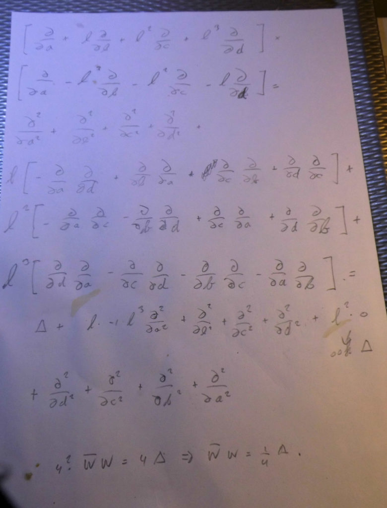
This year starting in January I found more and more counter examples to the last theorem of Fermat. As a by product when we looked at the stuff on the 4D complex numbers, we found that if we restrict ourselves to the 4D rationales, they were always invertible. And as such they form a field, this is a surprising result because the official knowledge is that the only possible 4D number system are the quaternions from Hamilton. So how this relates to those stupid theorems of Hurwitz and Fröbenius about higher dimensional complex numbers is something I haven’t studied yet. But that Hurwitz thing is based on some quadratic form so likely he missed this new field of 4D complex rationales because the 4D complex numbers are ruled by a 4 dimensional thing namely the fourth power of the first imaginary unit equals minus one: l^4 = -1.
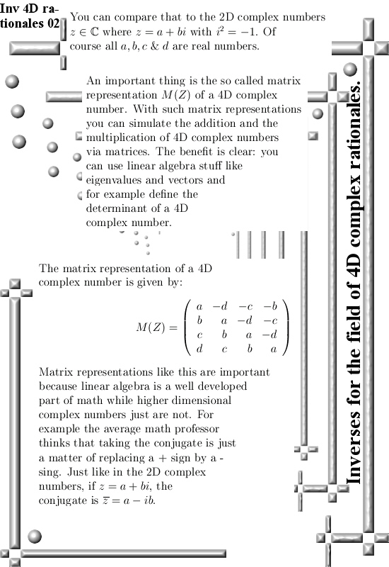
Compare that to the complex plane that has all of it’s properties related to that defining equation i^2 = -1.
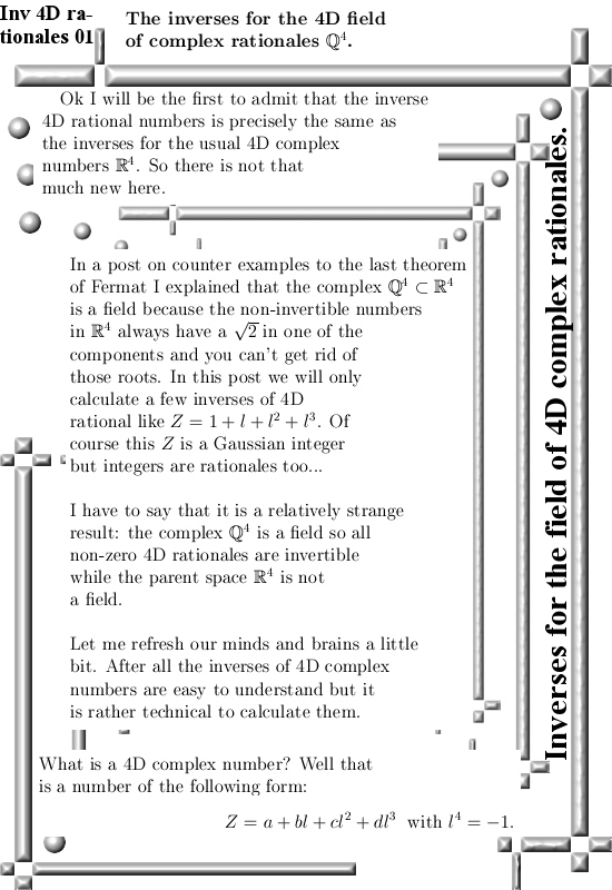
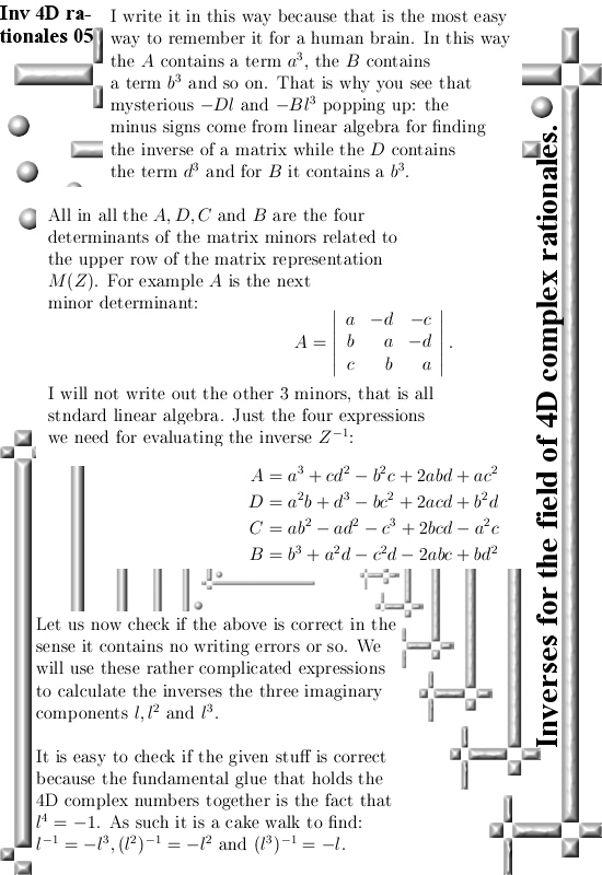
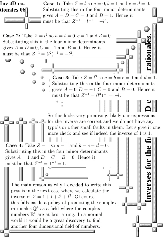
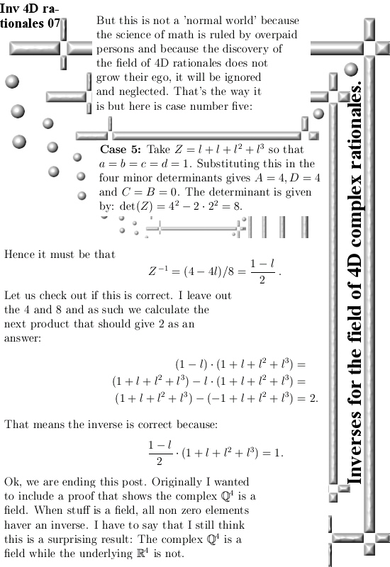
And because we now have a 4D field I thought like let’s repeat how you find the inverse of a 4D complex rational number. And also prove that we have a field as basic a proof can be. But while writing this post I had to abandon the second thing otherwise this post would grow too long. Of course in the past I have crafted a post for finding the non-invertible 4D complex numbers but in that post I never remarked that rational 4D complex numbers are always invertible. To be honest in the past it has never dawned on me that it was a field, for me this is not extremely important but for the professional math people it is.
When back in Jan of this year I found the first counter example to the last theorem of Fermat I was a bit hesitant to post it because it was so easy to find for me. But now four months further down the time line I only found two examples where other people use some form of my idea’s around those counter examples and both persons have no clue whatsoever that they are looking at a counter example to the last theorem of Fermat. But in a pdf from Gerhard Frey (that is the Frey from the Frey elliptic curve that plays an important role in the proof to the last theorem of Fermat by Andrew Wiles) it was stated as:
(X + Y)^p = X^p + Y^p modulo p.
That’s all those professionals have, it is of a devastating minimal content but at least it is something that you could classify as a rudimentary counter example to the last theorem of Fermat. It only works when your exponent if precisely that prime number p and it lacks the mathematical beauty that for example we have in expressions like:
12^n = 5^n + 7^n modulo 35.
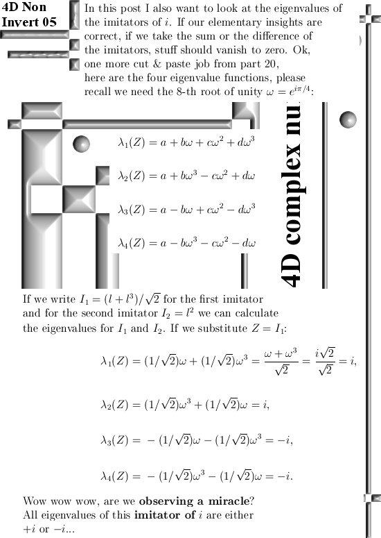
Anyway this post contains nothing new but there is some value in repeating how to find inverses of higher dimensional complex numbers. All you need is a ton of linear algebra and for that let me finish this intro on a positive note: Without the professional math professors crafting linear algebra in the past, at present day for me it would be much harder to make progress in higher dimensional complex numbers. And it is amazing: Why is linear algebra relatively good while in higher dimensional number systems we only look at a rather weird collection of idea’s?
This post is made up of seven pictures each of size 550×800 pixels.
Ok ok this post is not loaded with all kinds of deep math results. But if you have a properly functioning brain you will have plenty of paths to explore. And the professional math professors? Well those overpaid weirdo’s will keep on neglecting the good side of math and that is important too: That behavior validates they are overpaid weirdo’s…
For example the new and improved little theorem of Fermat: The overpaid weirdo’s will neglect it year in year out.
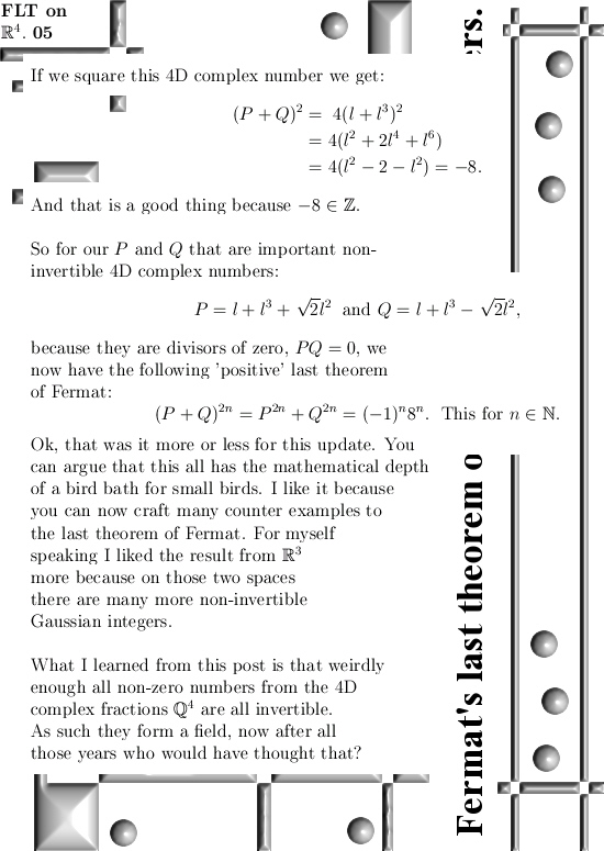
That’s the way it is, here is once more a manifestation of the new and improved little theorem of Fermat:

Let’s leave it with that. Thanks for your attention.