It is past midnight, this evening I brewed hopefully a lovely beer. It is late so let me keep the intro short. The last time I often lack stuff for new posts because most of the theory of 3D complex and circular numbers has been posted in this collection of 200+ posts. And you cannot keep it repeating over and over again, if all those years in the past the math professionals did just nothing, why would they change their behaviour in the future? Beside that I do not want have anything to do with them any more, it is and stays a collection of overpaid weirdo’s and there is nothing that can change that.
On the other hand one of the most famous expressions in math is and stays the exponential circle in the complex plane.
That stuff like e^it = cos t + isin t is what makes many hearts beat a tiny bit faster. So when someone comes along stating that he found an exponential circle in spaces like 3D complex numbers, you might expect some kind of attention. But no, once more the math professionals prove they are not very professional. Whatever happens over there I do not know. May be they think because they could not find this in about 350 years no one can so it must all be faulty. For me it was a big disappointment to get discriminated so much, on the other hand it validates that math professors just are not scientists. Ok they have their salary, their social standing, their list of publications and so on and so on. But putting lickstick on a pig does not make it a shining beauty, it stays a pig. So a math professor can have his or her prized title of professor, that does not make such a person a scientist of course. At best they show some form of imitating how a scientist should behave but again does such behaviour make these people scientists?
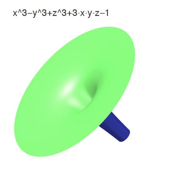
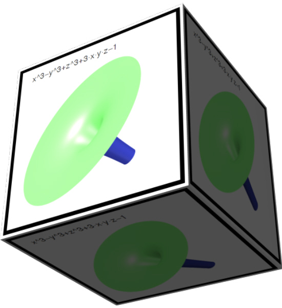
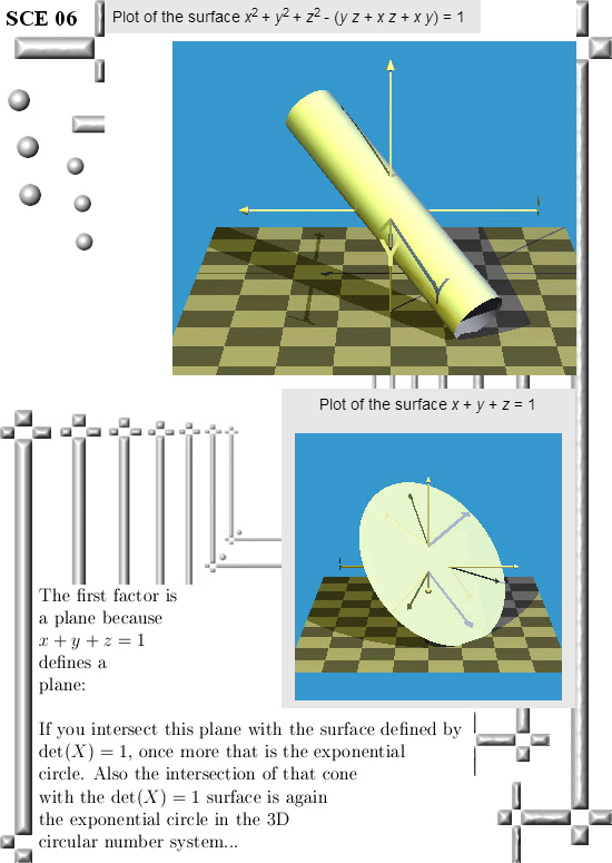
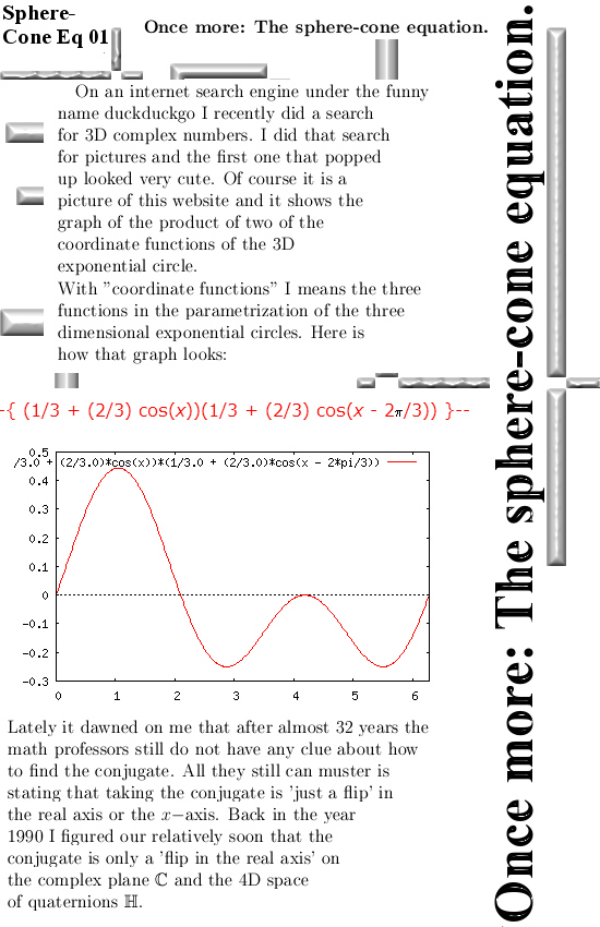
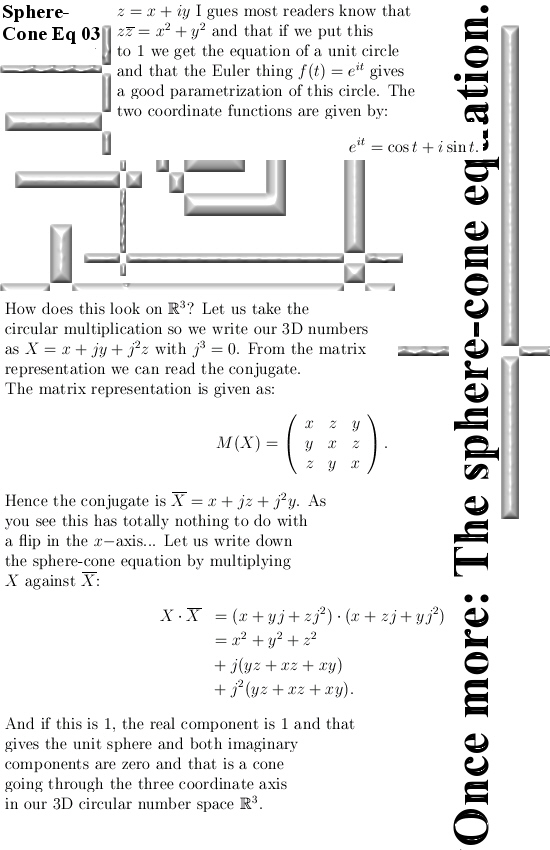
Anyway a couple of days back at the end of a long day I typed in a search phrase in a website with the cute name duckduckgo.com. Sometimes I check if websites like that track this very website and I just searched for “3D complex numbers”. The first picture that emerged was indeed from this website and it was from the year 2017. I looked at it and yes deep in my brain it said I had seen it before but what was it about? Well it was the product of two coordinate functions of the exponential circle in 3D. It is a very cute graph, you can compare it to say the product of the sine and cosine function in the complex plane.
So I want to avoid repeating all that has been written in the past of this website but why not one more post about the 3D exponential circles?
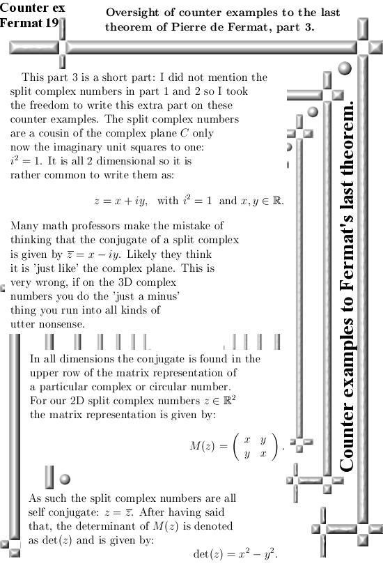
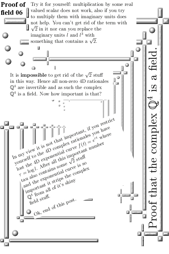
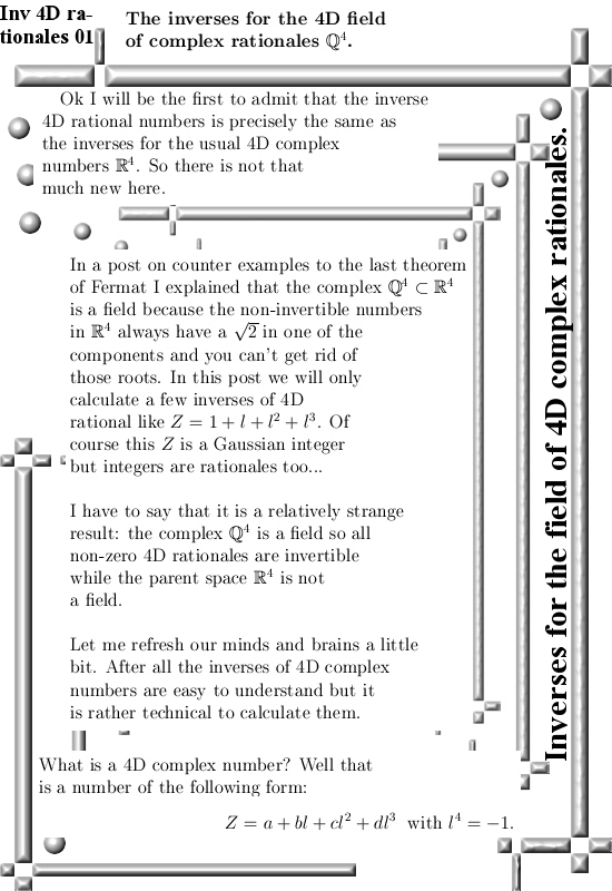
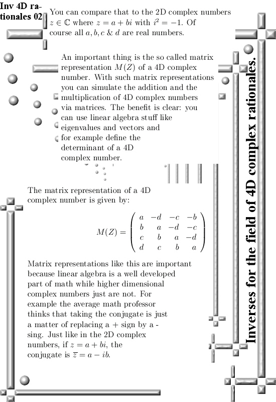
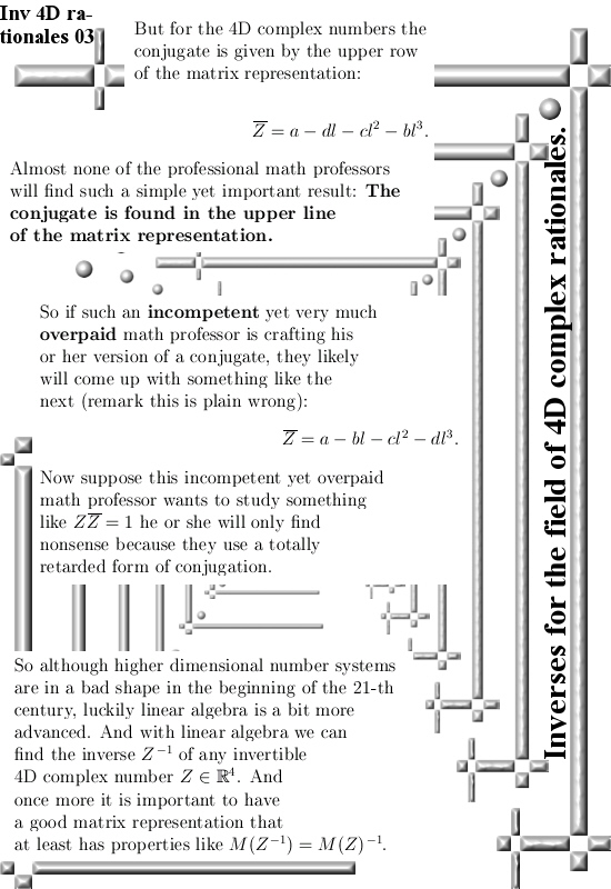
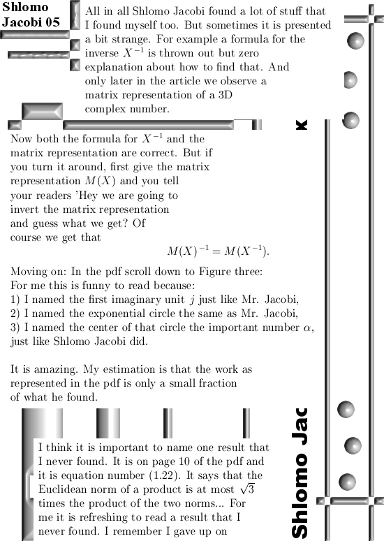
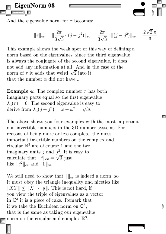
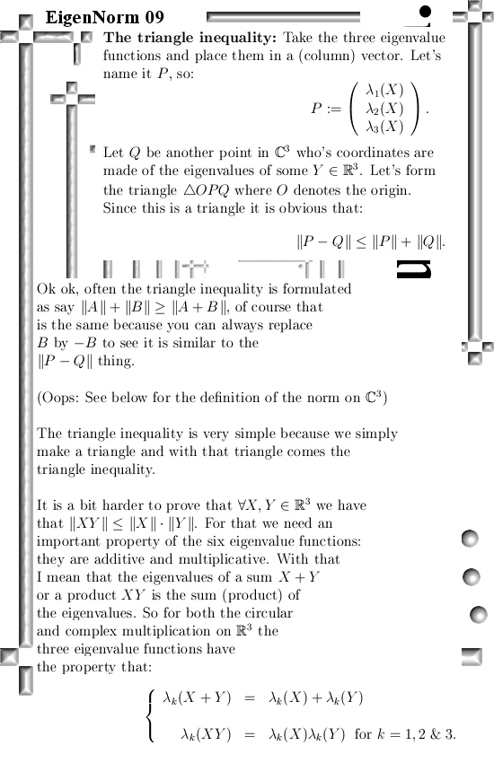
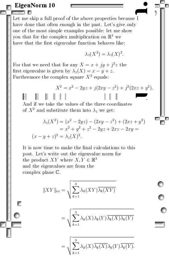
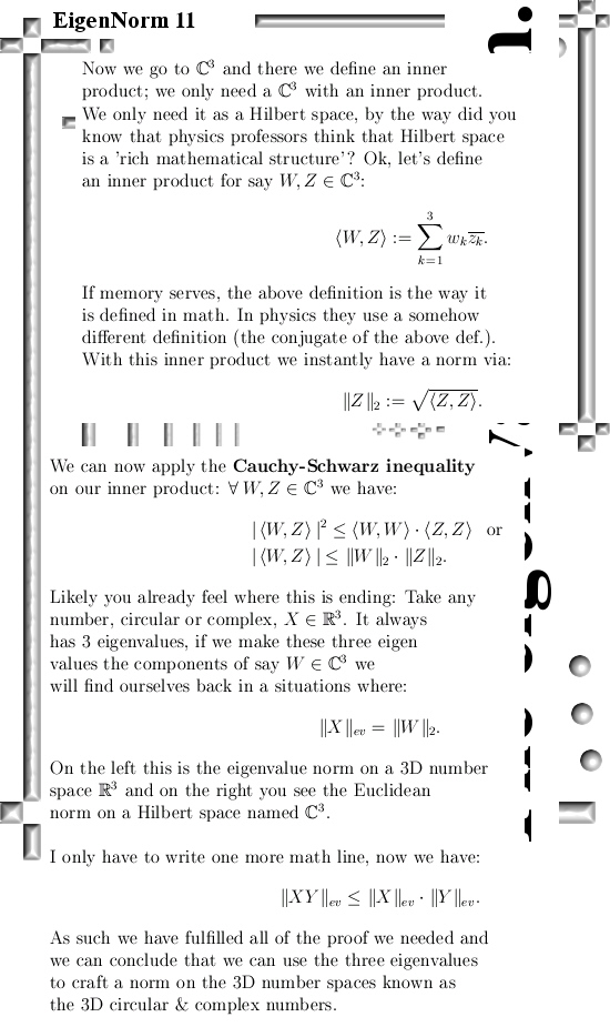
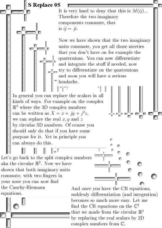
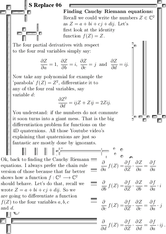
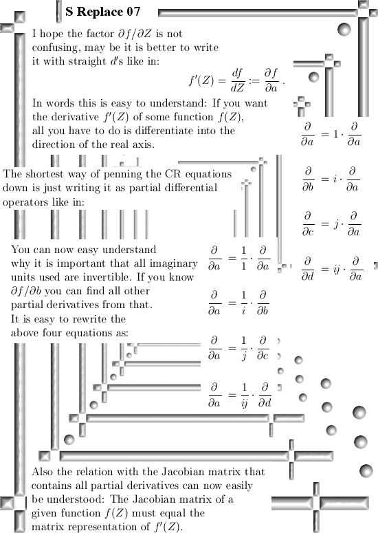
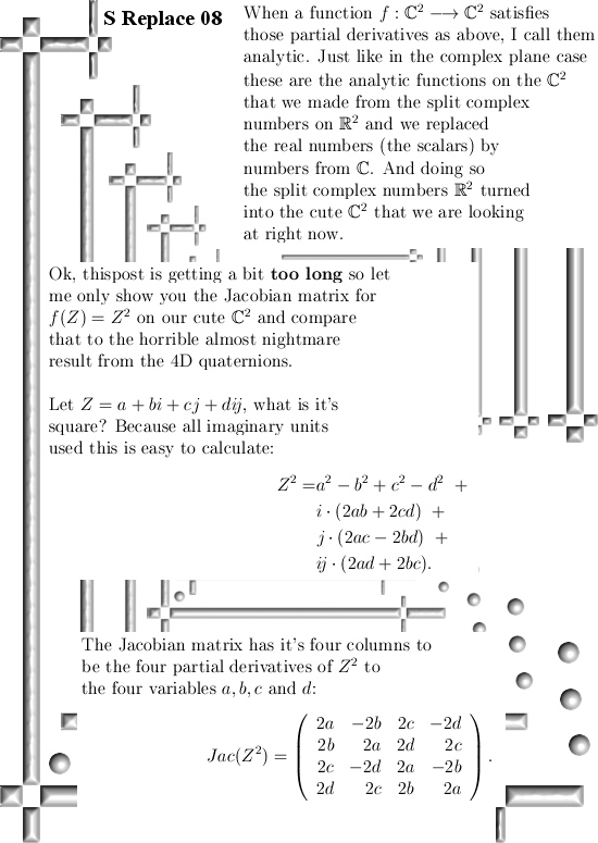
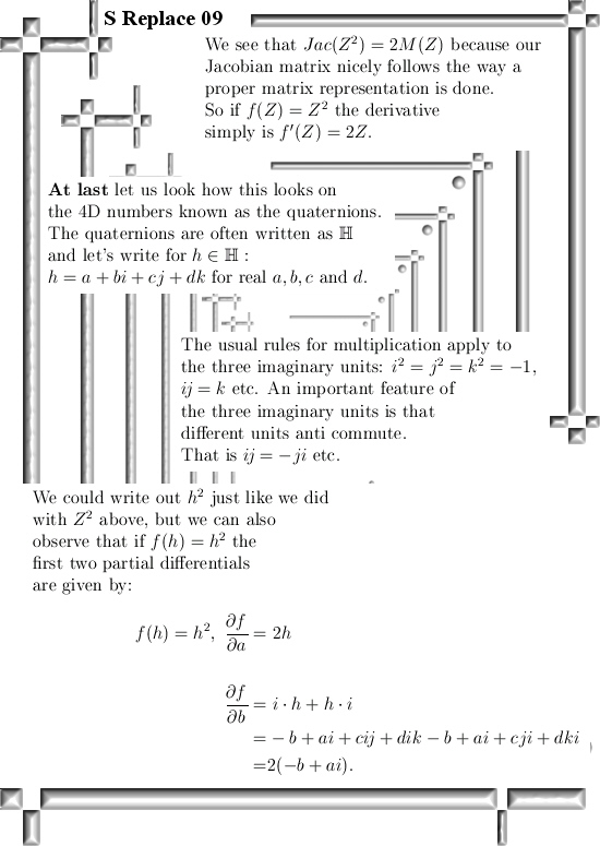
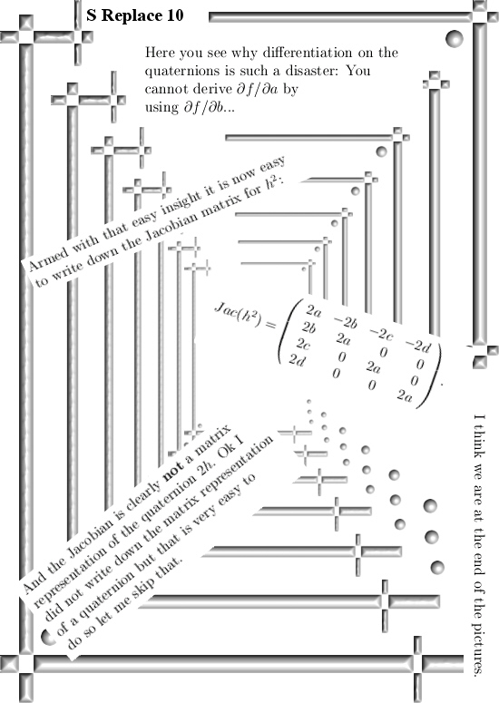
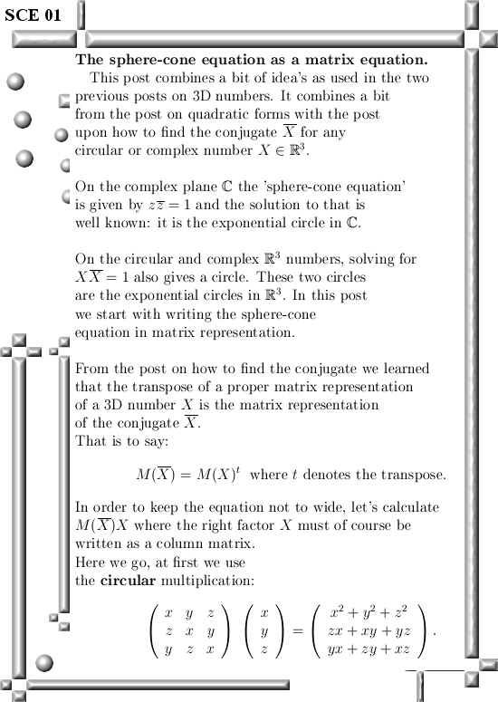
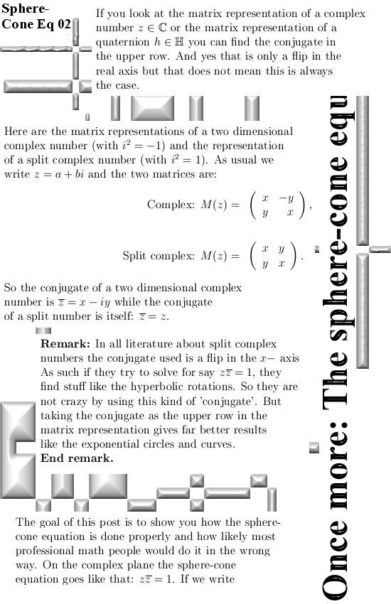
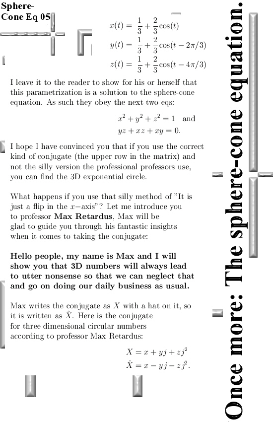
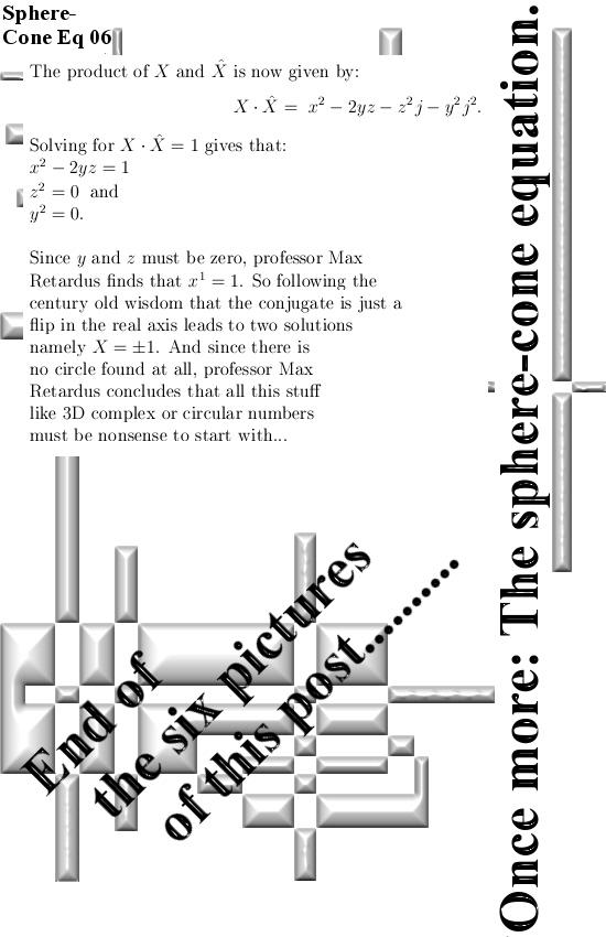
In the end I decided to show you how likely one of those deeply incompetent “professional” math professors would handle the concept of conjugation. Of course one hundred % of these idiots and imbeciles would do it as “This is just a flip in the real axis or in the x-axis” and totally spoil the shere-cone equation and only find weird garbage that indeed better cannot be published. After all our overpaid idiots still haven’t found the 3D complex numbers, I am still living on my tax payer unemployment benefit and life, well life will go on. But it is not only math, with physics there are similar problems and they all boil down to that often an idiot does not realize he or she is an idiot.
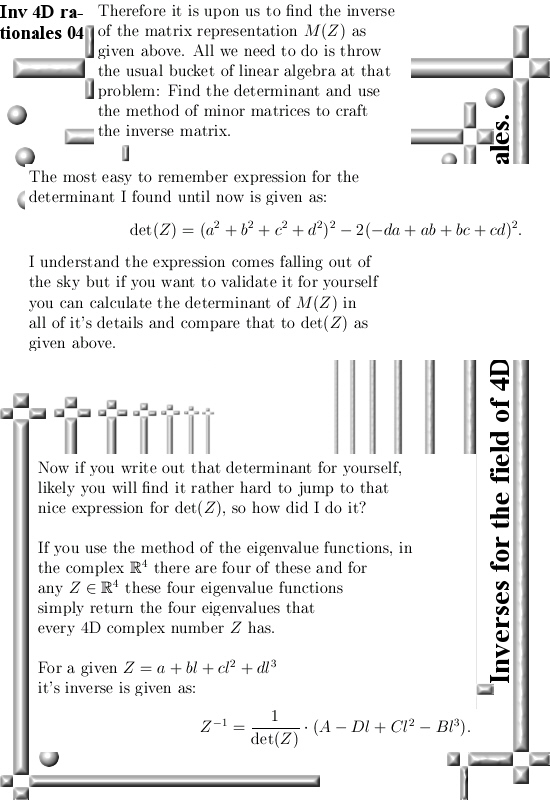
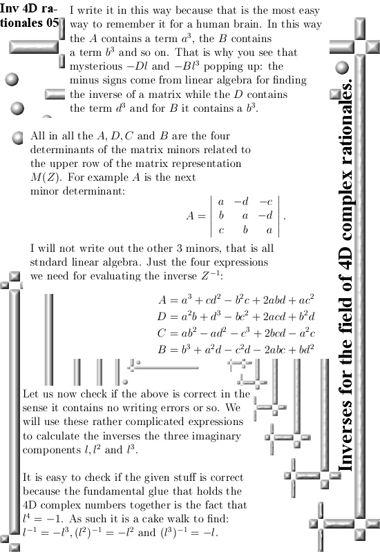
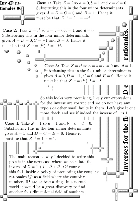
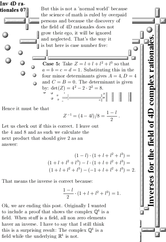
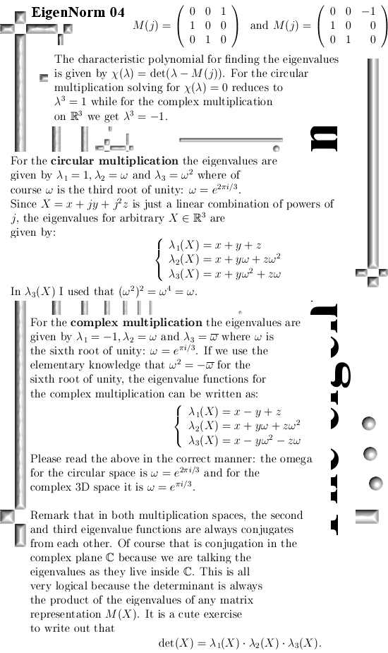
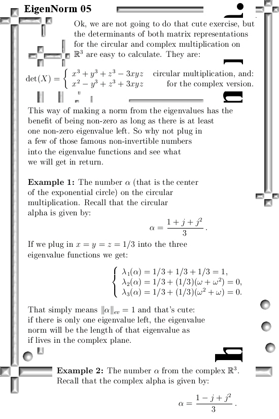
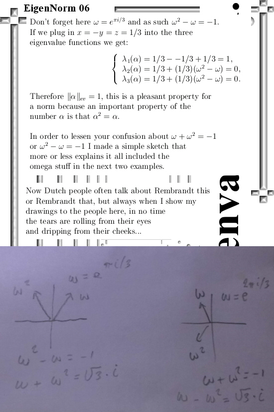
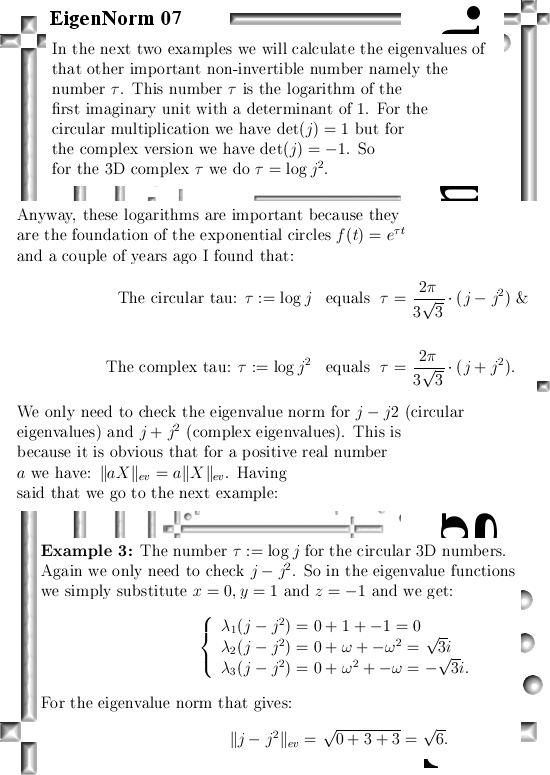
But let’s post the six pictures, may I will add an addendum in a few days, may be not. Here we go:
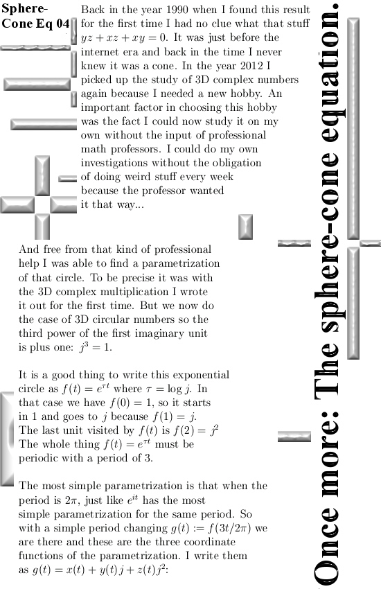
Ok, may be in will write one more appendix about how these kind of coordinate functions of exponential circles give rise to also new de Moivre identities. That is of interest because the original de Moivre identity predates the Euler exponential circle by about 50 years.
Yet once more: Likely there is just nothing that will wake up the branch of overpaid weirdo’s known as the math professors…
So for today & late at night that was it.
Thanks for your attention.