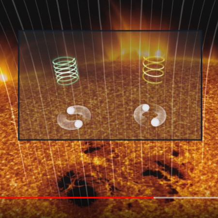
Oops I likely made a many year mistake when it comes to the magnetic stuff. Many years ago I had the idea that the magnetism as found in sun spots could possibly explained by spinning plasma underneath the solar surface. After all if electrons are magnetic monopoles, a spinning cylinder shaped plasma should eject lots of electrons along it’s magnetic field lines. That makes the spinning plasma a terrible good magnet because is a lot of positive charged plasma is spinning that creates strong magnetic fields.
After the original idea it took me about one year there could be a possible mechanism on the sun that creates such spinning plasma structures: The sun rotates faster at the equator as it does at the poles.
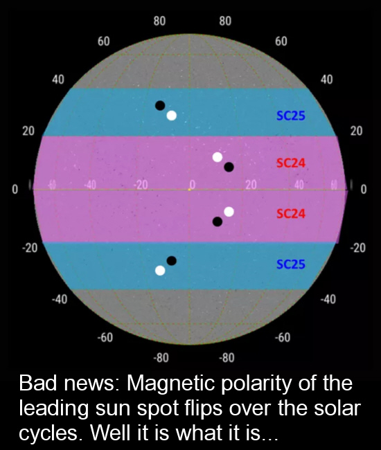
Now sun spots often come in pairs with opposite magnetic polarity and in my view I thought the leading sun spot was the one created by a bunch of rotating plasma under it.
It is easy to understand that if the root couse of sun spots was a rotating column of plasma underneath them, on the opposite hemispheres of the sun the leading sun spot should have opposite magnetic polarity. That one always checked true, but for the rotational hypothesis to be true over the solar cycles the polar magneticity of the leading sun spot should always be the same.
And that is where likely my old idea is crashing right now. In the next picture you see what is more or less observed in the last change of the solar cycle, for me this is not funny.
SC24 and SC25 stand for Solar Cycle 24 & 25 and again: for me this is not funny:
Yes it is what it is. But at least as soon as I discover I have made a serious mistake I tell that as soon as possible. All in all this mistake does not have any impact on the tiny fact that it is impossible for electrons to be tiny magnets, electrons are magnetic monopoles and as such we have two variants of them. So the Gauss law for magnetism is just not true for an individual electron, it is nonsense to say magnetic field lines always loop in on themselves.
But after seven years of explaining this kind of mistakes, that stuff known as the science of physics is not capable of cleaning herself of stupid ideas.
Let’s leave it with that, this correction is a set back but the weirdo’s classified as the physics professors still have to give some experimental proof that electrons are indeed ‘tiny magnets’.
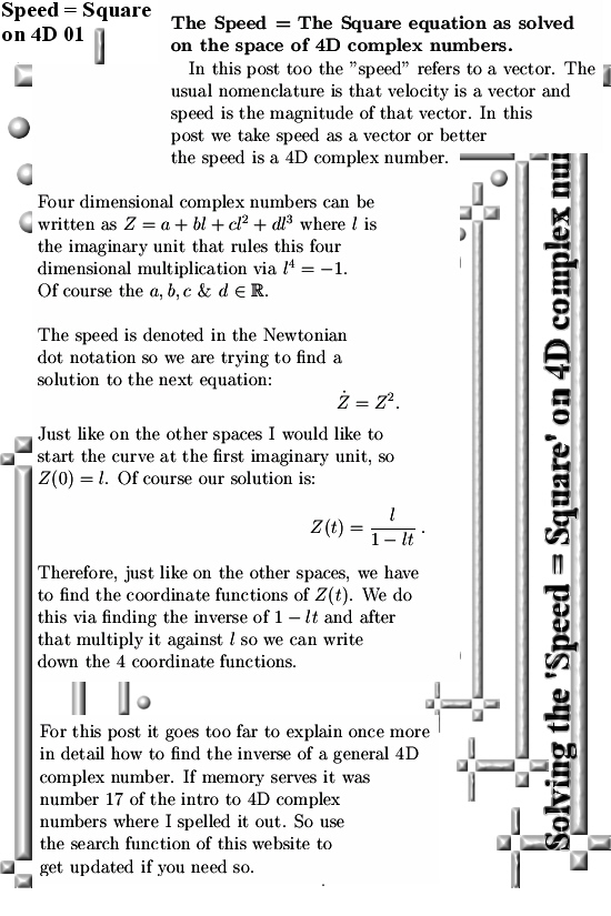
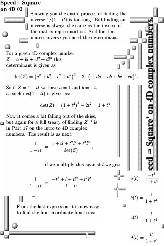
Unavoidable I had to write some post after the video on the quaternion from Hamilton. Now my 4D complex numbers commute so they are very different from the standard version of quaternions. Just like in the complex plane the multiplication is ruled by the imaginary unit i that has the defining property of i^2 = -1. On the space of four dimensional complex number I mostly write l for the first imaginary component, the defining property is of course that now the fourth power equals minus one: l^4 = -1. In 2018 I wrote about 20 introdutionary posts about the 4D complex numbers. That is much more as you would need for the quaternions of Hamilton but on the quaternions you can’t do complex analysis and that explains almost all of the difference. You can view the quaternions as three complex planes fused together by the common use of the real line. My 4D complex numbers can be viewed as a merge of two complex planes in the sense that there are two planes clearly ‘the same’ as a complex plane. This post is once more one of the ‘Speed = the Square’ equations and just as on the other spaces we looked at we choose the initial condition such that it is the first imaginary unit l. As such our solution is easily found to be f(t) = l / (1 – lt) because if you differentiate that you get the square. So from the mathematical point of view this is all rather shallow math because all we have to do is find the four coordinate functions of our solution f(t). For that you need to calculate the inverse of 1 – lt and to be honest after so much years I think almost all math professors are just to fucking stupid to find the inverse of any non real 4D compex number Z let alone if you have something with a variable t in it like in 1/(1 – lt).
I did my best to write this as transparant as possible while also keeping it as short as possible. For an indepth look at how to find the inverse of a 4D complex number, look for Part 17 in the intro series to the 4D complex numbers. (Just use the search function for this website for that.)
This post is just three pictures long so lets hope that is inside your avarage attention span. And it’s math so without doubt a lot of people will digest this with a speed of one picture a week! No I am not being sarcastic or so, I just like as how I evolved to the math place I am now. Often that also goes very slow but it has to be remarked the math professors are much more slow slow slow because they could not find the 3D complex numbers in all of human history. Let’s dive into the picture stuff:
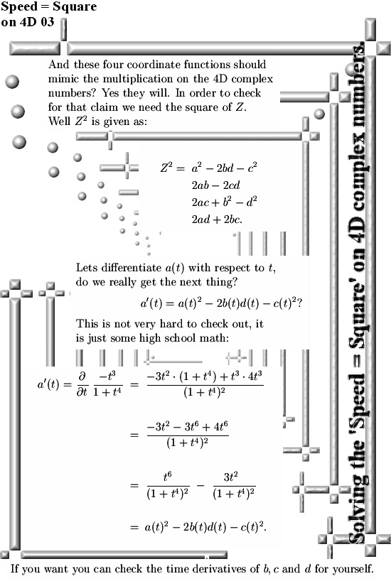
One of the funny things of the math of this post is that on the one hand it is very simple: You only need high school math like the quotient rule for checking my claims are true and differentiation mimics the multiplication on the 4D complex numbers. On the other hand you have those math professors likely not capable of finding these easy coordinate functions for themselves. But this post is not meant as an anti math professor rant but more upon the beauty of simple math you can do on say the space of 4D complex numbers. See you in the next post.
This very short post was written because of a video from the video channel Kathy loves physics. It is one of those “Quaternions are fantastic” video’s. And Kathy just like a lot of other physics people think indeed that quaternions are fantastic. But you cannot differentiate or integrate on the quaternions so I guess this stronly limits it’s use in physics. But quaternions are very handy in describing rotations in 3D space, I never studied the details but it was said that on the space shuttle it was used for nagvigation. And because of these rotation properties at present day they are used in the games industry.
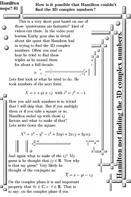
Anyway in the video Kathy explains that Hamilton did try for a long time to find the three dimensional complex numbers. And he never succeeded in that. Of course I know this for decades right now but in the past I never looked into a tiny bit more detail in what Hamilton was actually doing. And he was looking at complex numbers of the form X = x + yi + zj where the imaginary components both equal to minus one: i^2 = j^2 = -1.
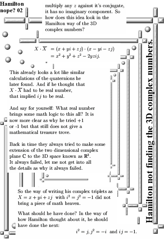
If you check the easy calculations in this post for yourself, it is amazing how much it already looks like the stuff as found on the quaternions. As such it is all of a sudden much less a surprise that Hamilton found the quaternions. As a matter of fact it was only waiting until he would stumble across them. But at the time the concept of a four dimensional space was something that made you look like a crazy lunatic, there were even vector wars and lots of crazy emotional stuff.
At present day it is accepted that 3D complex numbers do not exist, in my experience the professional math community is still emotionally laden but now into the direction of total neglect. Stupid shallow thought like “If Hamilton could not find them, they likely don’t exist”.
Back in the 19-th century they were always looking for an extenstion of the complex plane to three dimensional space. Of course they failed in that attempt because it is a fact of math life that you cannot solve the equation X^2 = -1 on the space of 3D complex (and also circular) numbers.
The content of this post is just two pictures, after that two more pictures as I used them on the other website and after that you can finally dive into the Video from Kathy. If you are interested in physics and also the history of physics, Kathy her channel is a thing you should take a look at if you’ve never seen it. Here we go:
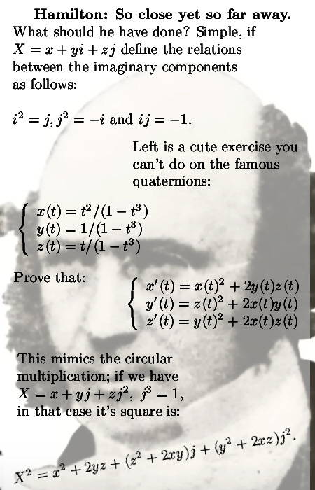
YES, that is what he should have done. Hamilton tried for about one decade to find the numbers that form the title of this very website, so may be he tried this kind of approach. I don’t know, but the 3D complex numbers are not some extension of the complex plane because 2 is not a divisor of 3. You know that prime number stuff is going on here. But the math professors are not interested in that kind of stuff.
Here is how I used it on the other website:
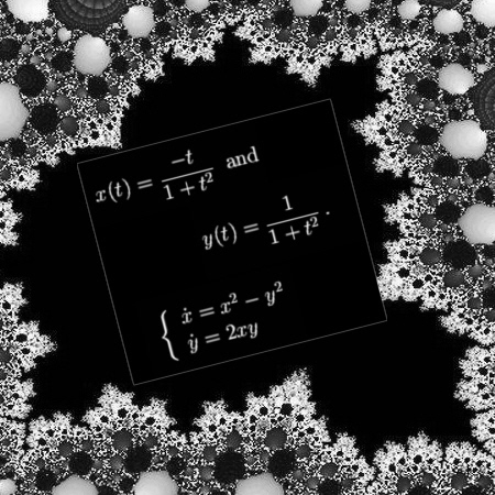
As you see in the above picture I was already working on the previous post because if you differentiate the three functions that mimics the 3D circular multiplication. You can also mimic the multiplication on the complex plane, that is in the next picture:
At last you can view the famous video of Kathy! It’s only 30 minutes or so but if you see too many so called TIKTOK videos that is infinitely long: Wow 30 minutes long looking at just one video?
End of this post, likely the next post is about 4D complex numbers.
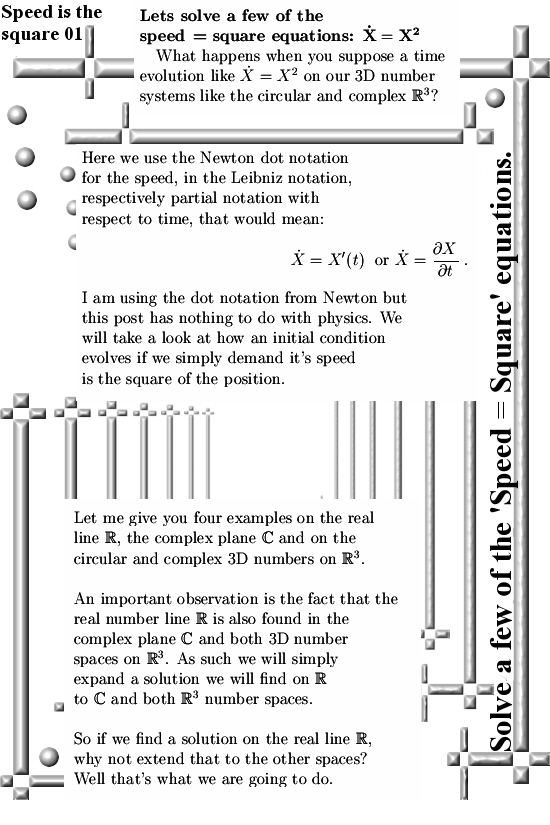
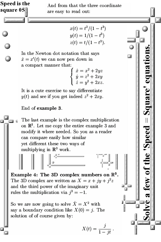
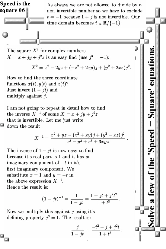
With ‘speed = square’ I simply mean that the speed is a vector made up of the square of where you are. The four spaces are: 1) The real line, 2) The complex plane (2D complex numbers), 3) The 3D circular numbers and 4) The 3D complex numbers.
I will write the solutions always as dependend on time, so on the real line a solution is written as x(t), on the complex plane as z(t) and on both 3D number spaces as X(t). And because it looks rather compact I also use the Newtonian dot notation for the derivative with respect to time. It has to be remarked that Newton often used this notation for natural objects with some kind of speed (didn’t he name it flux or so?). Anyway this post has nothing to do with physics, here we just perform an interesting mathematical ecercise: We look at what happens when points always have a speed that is the square of their position.
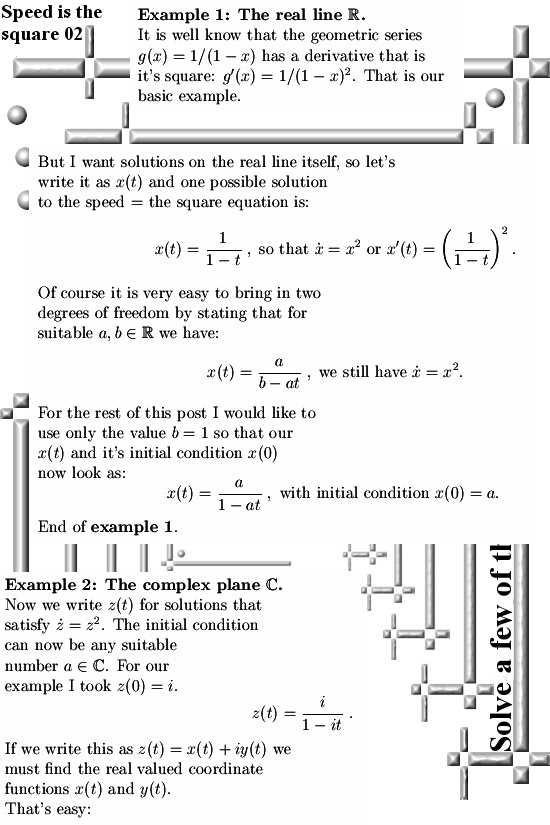
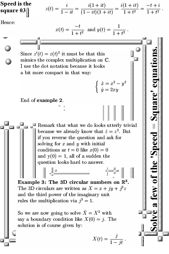
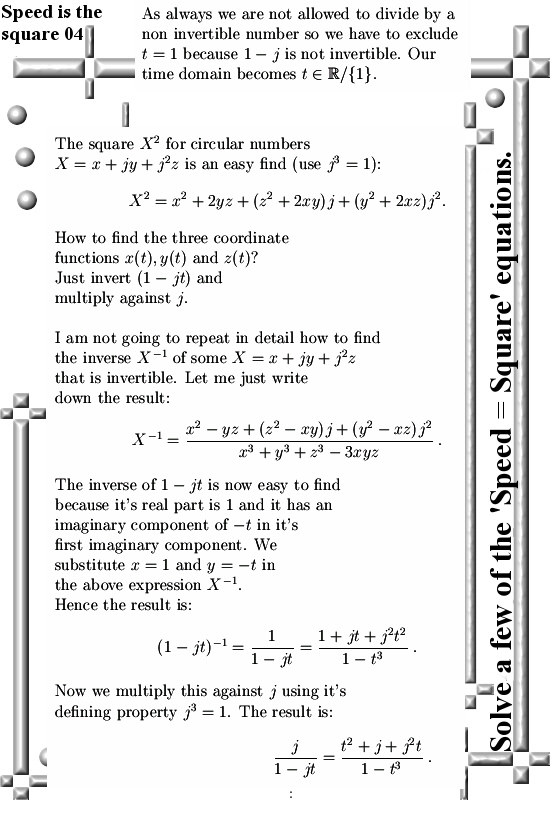
On every space I give only one solution, that is a curve with a specific initital value, mostly the first imaginary component on that space. Of course on the real line the initial condition must be a real number because it lacks imaginary stuff.
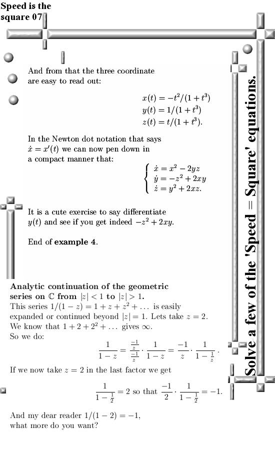
If you go through the seven pictures of this post, ask in the back of your mind question as why is this all working? Well that is because the time domains we are using are made of real numbers and, that is important, the real line is also a part of the complex and circular number systems. The other way you can argue that the geometric series stuff we use can also be extended from the real line to the three other spaces. To be precise: we don’t use the geometric series but the fractional function that represents it.
Ok, lets go to the seven pictures:
That Newton dot notation just looks so cute…The words ‘Analytic continuation’ are not completely correct…
Remark: This post is not deep mathematics or so. We start every time with a function we know that if you differentiate it you will get the square. After that we look at it’s coordinate functions and shout in bewilderment: Wow that gives the square, it is a God given miracle!
No these are not God given miracles but I did an internet search on the next phrase of Latex code: \dot{z} = z^2. To my surprise nothing of interest popped up in the Google search results. So I wonder if this is just one more case of low hanging math fruits that are not plucked by math professors? Who knows?
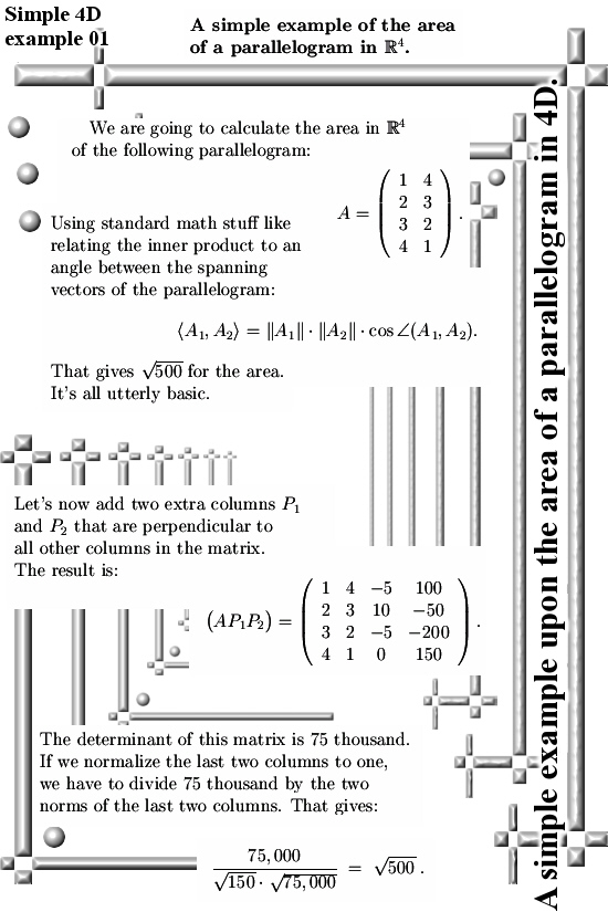
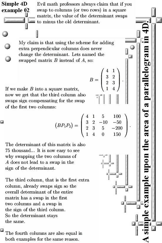
This is one of the details I should have posted last year. So this post is some mustard after the meal. The content is just two pictures long. In it I show you how to calculate the area of a parallelogram in 4D space. After that we swap the two columns and use the same method again. In both cases the area of the parallelogram equal the square root of 500. If you read stuff from this website you likely have enjoyed some classes in linear algebra, likely you know that if you swap two columns (or two rows) in a square matrix, the determinant changes sign. But the way we turn a non-square matrix into a square matrix is done in such a way that it has to return a positive (or better: non-negative) number. In this example you can see that if you swap the two spanning columns of the parallelogram, the first extra column or the third column in our final matrix also chages sign. So the overall determinant of the 4×4 final matrix ‘observes’ a swap in the first two columns and also a swap in the sign of the third column. Hence the determinant does not change sign…
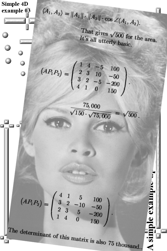
Originally I only needed a few cute looking formulas for use on the other website. That are the two matrices below. But when finished I added some text and as such we have a brand new post for this website.
In this example I did not normalize the extra columns to one so if you want you can play a bit with it and as such observe how their norms are related to the area of the diverse parallograms in here. For example if you calculate the norm of the fourth column, it is the square root of 75,000 while the determinant of the whole 4×4 matrix is 75,000.
As such constructing square matrices like this always leads to the last column having a norm that is the square root of the determinant. That is a funny property, or not?
Anyway here are the two pictures, the third picture is an illustration of how it was used on the other website. As usual all pictures have sizes of 550×825.
In the third picture I used an old photo of Brigitte Bardot as a background picture. Now both Brigitte and me we looked a lot more fresh back in the time from before they invented the stone age. Our minds were sharp and our bodies fast while at present day we are just another old sack of skin filled with bones, fat and some muscle. Life is cruel..
Ok, lets end this post now and see you around my dear reader.
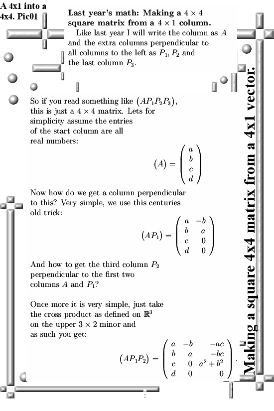
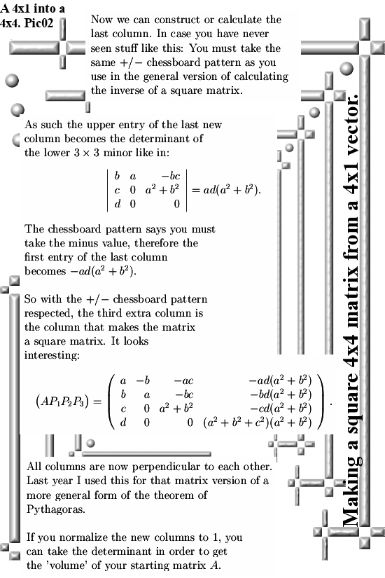
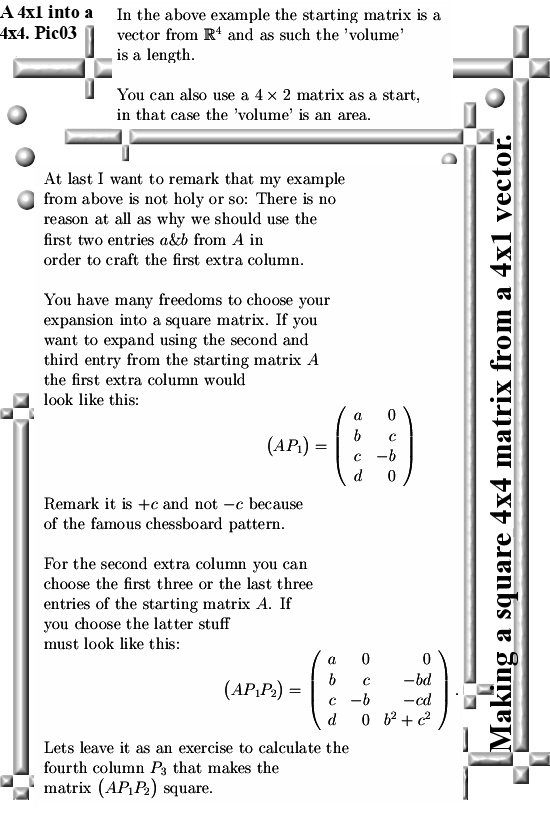
Yes I know that two posts back I said that this would be the last time we would do Pythagoras stuff like this. On the other hand I was very unsatisfied with that post (title: That weird root formula). Also I had wanted to post the math below before but I did not have the time. All in all since I was horribly bad in the post upon that weird root formula about how to make extra columns, may this short post compensates a bit for that. This post starts with a column of four real numbers, say a, b, c and d. The goal is to keep on adding extra columns such that all columns are perpendicular to each other. Don’t confuse that with an orthogonal matrix, orthogonal matrices also have all their columns perpendicular but the columns are also all of norm one. For myself I name matrices that have all their columns perpendicular to each other ‘perpendicular matrices’ but this is not a common thing in math communications as far as I know. I show you two examples here: First I make an extra column based on the a and b entry of our vector. In the second expansion of the same vector I use the middle two entries b and c. This should serve as examples that make it as transparant as possible how you must use the +/- chessboard pattern that comes with calculations like this. For understanding this post it comes in very handy if you have done & understand the general way of crafting the inverse of a square matrix. I think most people will see the brilliant +/- chessboard scheme there for the first time in their lives.
I don’t know much about the history of math, but I like it that the +/- chessboard scheme has no human name attached to it like in “Hilbert space”. I guess this chessboard pattern emerged slowly over the cause of a few decades with contributions of many people. So in the end there was nobody to name it too because this big success just had to many fathers.
Another explanation for the lack of a human name to the famous +/- chessboard pattern is that the person who for the first time chrystal clear wrote out the stuff, this person was not an overpaid professional math professors. But say an amateur just like me. Well in those good old times just like now, the overpaid math professors can’t give credit to such an undesireable person of course… Yet not all is negative when it comes to professional math professors: They are still very good at telling anybody who wants to hear it that: “We tried but we could not find the three dimensional complex numbers”.
After all that human blah blah blah, why not take a look at the three pictures?
Please do that exercise so you can say you understand that +/- chessboard scheme.
A happy new year by the way, it is now 3 Jan over here so it is not too late to wish you that. So be happy if you can ask a physics professor or teacher as why there is no experimental proof at all that electrons are tiny magnets. And if the answer is not satisfactory, just chop the head of while being happy…;)
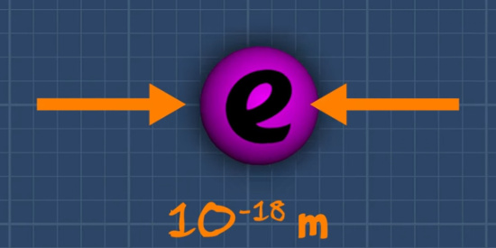
But serious, I selected the first video because the guy from the Science Asylum channel gives are very tiny estimated upper bound for the possible size of the electron: 10 to the -18 power meter as diameter. That is very very small, it is a nano nano meter.
Lets construct a so called ‘toy model’ for imitating in a simple manner how the electron is supposed to be a tiny magnet: Take two pointsize magnetic monopoles, a north and a south one and place them 10 to the power -18 meter apart. Lets name this distance d. An important feature of such a dipole is that it’s magnetic field declines inversely with the third power of d.
Let me give you an example: Take a line through the north and south pole of our toy electron and go out a distance of say 10d above the north pole. So the distance of our point on that line is 10d to the north pole and 11d to the south pole. The magnetic forces or field strength if you want is now proportional to 1/10^2 and 1/11^2. But north and south pole have opposite workings so we are looking at the difference: 1/10^2 – 1/11^2 and that is something of the order 1/1000.
If the electron diameter is indeed at most this distance d, in that case the two overlapping magnetic fields cancel each other almost out. If all that tiny magnet stuff is true, in that case the electron should be magnetically neutral. In a constant magnetic field that does not vary in space, by definition this tiny magnet electron should be neutral (if it all was true).
Let me show you two screen shots from the video from the Science Asylum. The first simple shows you the claim the electron has at most this size d.
On a nano nano scale this should be magnetically neutral…
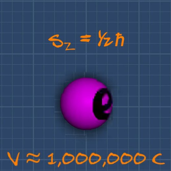
A long time ago I estimated the result in next picture too but I always used an electron diameter of 10 to the -16 power, so one hundred time as big as the Asylum guys claims. Anyway there is nothing spinning over there because it must rotate a huge multiple of the speed of light. Now we can honestly say that Albert Einstein did not understand much about electron spin, but we can safely conclude that electron spin is not related to rotation of a spherical charged body the size of d.
One million times the speed of light…
Ok, let me hang in the video where we have once more the implicit claim that magnetism is always a magnetic dipole without one iota of experimental proof for that claim:
In my view the most misleading name is spin, it sets your brain totally wrong.
In the next video you see a guy at work showing that the oxygen in the air you breathe is magnetic. The magnetic properties of oxygen are truly breathtaking because it has to do with a so called ‘non-binding’ electron pair. In chemistry a non-binding electron pair is a pair with the same electron spin. Weirdly enough the physics professors keep their mouth shut: All electron pairs obey the Pauli exclusion principle! Until it doesn’t like in molecular oxygen.
But I digress, the reason I selected this video can be found at 3.40 minutes into it: The guy ‘explains’ the behavior of the oxygen by stating that the two electrons in the non-binding pair align their magnetic dipole to the applied magnetic field. The problem with this kind of ‘explanation’ is that it does not explain as why the electrons get accelerated. As said above; if electrons are tiny magnetic dipoles, they are basically magnetically neutral. And we are to believe that the oxygen molecules get accelerated by the applied magnetic field because two little electrons ‘align their dipole magnetic moment’. Give me a break: that is crap and the next stuff look much more logical and observable: Electrons are not magnetic dipoles but magnetic monopoles.
Here is the second video:
The reason for posting this second video is that I often obverve people from physics thinking that the alignment or for that matter the anti-alignment explains the acceleration and forces involved.
After seven years into this stuff I only wonder:
Why do the physics professionals like teachers and professors not see they are telling utter crap? Why are they so fucking stupid all of the time? End of this post. Once more: A happy new year.
It took an amazing amount of time to finish this post. When I started it you could still bike in the city with your shorts on. And now it is freezing cold at the start of winter. I posted over 220 posts on this website but I never experienced such a long lasting writers block on my behalf.
I think the start was much to impulsive, mostly I take more time before I pick a subject for the next post. This time I did not do that and soon I ran into writers regret: Why did I start this BS that is far to complicated to explain in a few lines of writing?
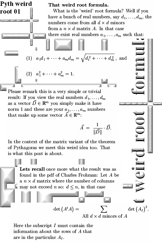
Even the beginning is dumb to do: It makes the reader think it is something solely on that space and it’s unit ball. And that dumb deed alone is a misrepresentation of what the weird root formula is about.
Anyway it is what it is and may be it is a good thing to show you that I can be very impulsive to. And in the science of math that is not a good thing.
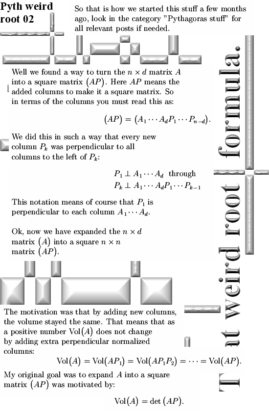
Since it has been a while I posted the last post on the matrix version of our beloved theorem of Pythagoras, readers who are new must use the search function on the website or just look into the category ‘Pythagoras stuff’. The matrix version of the Pythagoras theorem is not that hard to formulate but hard to prove. It goes like this:
Given some n x d matrix A made up of d columns, if the d columns are linearly independent this defines or represents a d-dimensional parallelapiped. What can be said about the d-dimensional volume, or better the square of this volume? It seems that the matrix A has lots of d x d minor matrices and if you take the determinant of these minors, square them they will add up to the desired square of the volume of A.
As you see: The result is not that hard to understand while our small human brain has trouble to cough up 20 proofs in 40 minutes.
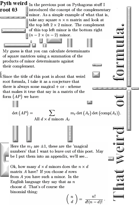
The key idea of the weird root formula is that you can apply an alternative way of calculating determinants: Multiplying determinants of minors against determinant of their so called complement. So for the matrix A that should give it’s d-dimensional volume.
But if you expand the matrix A with an extra column perpendicular to all columns of A, say you get AP_1 and of course you normalize P_1 to length 1, you can repeat the whole thing on the expanded matrix. This goes on until the matrix A has been made a square matrix that I denote as AP. In this post I use the notation (AP) for the square matrix so you must never view AP as the product of two matrices or so because that is not what it is…
This post if four pictures long but it has to be remarked I skipped how to find that +/- scheme you need for calculating determinants this way.
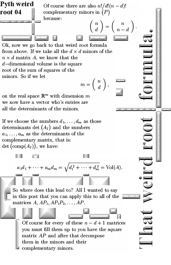
So after all this time this Pythagoras stuff is published. All in all it is a cute idea, that weird root formula can be applied not only to that starting matrix A but also on every extension with extra perpendicular columns.
In the last seven years it has taken me a long time to arrive at the conclusion that electron spin is a permanent property of electrons. The only place in this universe where electrons get their spin flipped is in the head of physics professors. For new readers: The last years I work from the hypothesis that electrons are magnetic monoples but every now and then I still try to kill that idea. But I always fail, in the end the electrons having a monopole magnetic charge always wins it from models like the ‘tiny magnet’ model for electrons. Why took it so long for me to finally accept this ‘permanent’ status of electron spin or as I say it: electron magnetic charge? Well there are a lot of video’s out there where people from physics explain how they flip electron spin while building quantum computers. At the end I post a long video from a guy named Lieven Vandersypen who works at the Technical University in Delft. Now I do not hate these people but when I say for seven years on a row ‘Where is you experimental proof that electrons are indeed tiny magnets?’. If seven years on a row just nothing happens over there we can safely conclude that Mr. Vanderlieven is just another UI. And an UI is a person that is an Ultimate Idiot or if you want an Ultra Ignorant.
In the theory of quantum mechanics before a measurment is done, it is assumed that a quantum particle is in a superposition of all possible states the quantum particle can be in.
Physics professors think that all electrons are the same and as such it has to be that before the measurement of the electron spin it is always in a superposition of spin up and spin down.
Remark this is very different from what I think: If the monopole magnetic charge is permanent, repeated measurments should always give the same magnetic charge. Just like measuring the electric charge of an electron always returns that is has one unit of negative electric charge…
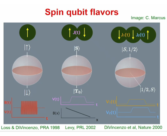
In the present hype of building quantum computers, almost 100% of the physics people think that it is possible that the electron is in some super position of spin up and spin down. I think this is not possible because we are having two different kind of electrons in this universe. If true you can wonder how far astray physics has driven from reality; in the next screen shot you see Mr. Vandersypen wonder what kind of qubit is the best for quantum computing. He says that they have been wondering for years what basic configuation of electron spins as qubits is the best. They think that every electron can be in a super position of spin up and spin down. On top of that if you have an electron pair they think it is in a super position of spin up-down with spin down-up, that is that Bell stuff.
If my view on electron spin is correct, all these approaches in quantum computing will never work. Here is how these fantasies look:
Now have you ever heard of an electron triple like in the right of the above picture? Why are there only electron pairs or unpaired electrons found in nature? That is because electrons are magnetic monopoles and that is why the electron pair is magnetically neutral while the unpaired electron is not magnetically neutral.
Compare that to the electric charge of the hydrogen atom. All in all it is neutral because the electric charges cancel each other out. So you can’t accelerate atomic hydrogen with electric fields until the electric field gets so strong it rips apart the hydrogen atoms. So why are electrons accelerated by magnetic fields and electron pairs not? After all if the electrons are ‘tiny magnets’ are they not supposed to be neutral when it comes of magnetic fields?
The title of this post says I have to give you some reasons as why electron spin or magnetic charge is permanent. So lets try a bit:
Reason 1) The official version of electron spin is that if you measure it in one direction, say the direction of an x-axis in a 3D coordinate system, that gives a reset for measuring electron spin in perpendicular directions say the y and z-axis. But any interaction with a magnetic field is a measurement in some direction. So these weirdo’s try to tell us that electron spin flips all the time because after all there are a lot of magnetic fields around us all the time. In the previous post I showed you the weird result that oxygen has a so called non-binding pair of electrons. That’s why it is magnetic. But molecular oxygen O2 is stable, if you apply magnetic fields to it no spin reset is observed. The non-binding pair does not change and all other electron pairs also don’t do weird stuff and the oxygen molecule stays stable under application of all kinds of magnetic fields.
Reason 2) The (hyper, see correction and addendum at the end) fine spectral structure of atomic hydrogen. There are very small differences in energy levels of the electrons in atomic hydrogen. The official version is that the electron spin and nuclear spins are aligned or anti-aligned. Of course it is never explained how an electrons supposedly going around the nucleus with high speed maintains it’s alignment… In my view where electron and proton spin are just magnetic charges, it is all blazingly simple: there must be four variants of atomic hydrogen when it comes to spin. Proton spin up or down combined with an electron with spin up or down. When both proton and electron have the same spin, the electron will be in that slightly higher energy level. And if the spins in atomic hydrogen are opposite, the electron has a bit lower energy because after all magnetic opposite monopoles attract.
Reason 3) A very interesting observation of the ESO (European Southern Observatory), it is about sun spots and different sun spots give different circular photons in the light coming from those sun spots. I have to collect more evidence that circular photons with opposite circular polarization are produced by electrons with opposite spins. But once more it has it’s own logic to it: If electrons are magnetic monopoles it is rather logical that the photons they produce have their magnetic fields shifted by 180 degrees. It is just like in the simple complex exponential from the complex plane: e^it = cos(t) + i*sin(t). As we all know this turns counter clockwise, now if we shift the sine by 180 degrees we get cos(t) – i*sin(t) and as we all know this rotates clockwise. This post is not meant for all the details that go into sun spots; it is more that after seven years of searching it is impossible to kill the idea that electrons are magnetic monopoles. It is a pity that physics professors are just dumb as hell when they say that electrons are ‘tiny magnets’ without any fucking experimental proof for such bold claims. The problem those people have is that they even think it is not a problem there is no such expemental proof. So these weirdo’s build giant theoretical structures like spin waves without proving the very fundamentals of their own science.
But lets not get emotional about the giant stupidity of physics professors, they even explain the giant magneto effect in a highly complicated way and that is funny. You can’t say they are scientists, at best they are weirdo’s trying to craft a theory of everything and of course such theories are all bullshit if electron spin is not done properly. Here is the ESO picture:
The leading sun spot should always have the same magnetic polarity just always… So it does not depend on the solar sun spot cycle.
It is about time to go to the video from Lieven Vandersypen and I have an extra video also from TU Delft where they explain the Majorana fermions. Relatively early in his video Lieven claims that there “Is nothing more a quatum bit than the spin of an electron.” Since in this post I try to explain that the only place in this universe where an electron flips it’s spin is in the head of physics professors like Lieven. It is impossible to have more contradiction as there is now between me Reinko and Lieven. In itself the video from Lieven is not that important, I only post it to show you one of those guys that believe electrons are tiny magnets while there is no experimental proof for that in the entire history of physics.
Video title: Lieven Vandersypen: Quantum simulation and computation with quantum dots – “spins-inside”
By the way in case you are interested: Lieven was the guy that years ago factored the number 15 in 3 times 5 using Shor’s algorthim. At present day we are standing at a factorization of say 21 in 3 times 7.
Back about one decade ago over there at TU Delft they thought they had found so called Majorany particles. These are particles that supposedly are there own anti-particle. That is a funny idea; if two of the same Majorana particles meet they anihilate each other. Why nature would produce such strange things is unknown to me. But if that Majorana shit is also based on electrons being ‘tiny magnets’, wouldn’t it be about time to try and prove via at least one experiment that electrons are tiny magnets?
Give me a break: university people actually using their brain? Please get a more realistic life…
Warning: This is not science! Keep away from children!
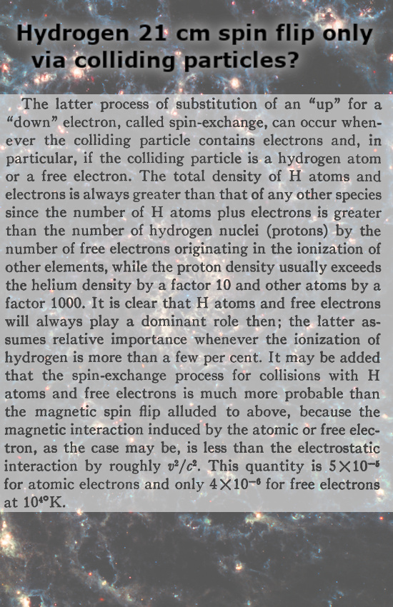
That was it for this post, once more since last year I do not try any longer to convince anybody that electrons are not tiny magnets. If the weirdo’s from Delft want tiny magnets if they look at electron behavior, what’s the problem with that? __________ Correction and addendum from 12 Dec: In reason 2 I named it ‘fine structure’ where it should read hyperfine structure of the hydrogen spectrum. So far for the correction. The addendum is a pdf from a 1958 article from the local university, the RUG. The old article is about spin flip in atomic hydrogen, it is about that famous 21 cm line in the hydrogen spectrum.
Now years ago when I was still very intimidated by big names like Mr. A. Einstein who had calculated the probability of a hydrogen atom to do the 21 cm transmission spontaneously. And who was I to say that electron spin was not a vector by a monopole magnetic charge and on top of that this charge was permanent just like the electric charge of an electron?
Back in time I had figured out that a collision with the right kind of electron of the right magnetic charge could also lead to this 21 cm emmision. The old electron of the hydrogen atom is simply replaced by a new one that binds in a somehow lower energy state.
To my surprise in the old article this is all covered in detail. If it is true that my idea of a permanent magnetic charge for the electron is correct, in that case 21 cm astronomy can more or less ‘see’ the galactic streams of electrons. After all if electrons are magnetic monopoles, the galactic magnetic fields play some role into what earth based astronomers see when they look at the 21 cm results.
In the next picture you can see the old text from 1958 while I use a new James Webb Space Telescope picture in the background:
It is funny that the local university has such an old article online…
Ok, left are a link to the pdf and the title of the old article:
Link used: https://www.astro.rug.nl/~saleem/courses/EoRCourse/Field1958.pdf
Ok now I promise you I will not place more updates or corrections on this post. It’s useless anyway, if I was impressed by Einstein just think about the consequences that has for physics professors… The weirdo’s will never stop thinking that you can flip the magnetic charge of an electron. They will never stop thinking you can flip electron spin.
I was watching a video about chiral chemistry and there it was explained that during the electrolysis of water if you coat the electrodes with some chiral coating, the efficiency is much higher. Now I was surprised but the explanation seems to be that oxygen has one so called non-binding electron pair. So that electron pair has two electrons with the same spin. Lately I found out that chiral molecules are able of electron spin selection, I have to admit I don’t understand just one tiny detail of how that works but on the other hand physics professors don’t understand electron spin. So compared to that I am doing fine. For readers who are relatively new: During the last 7 or 8 years I have been trying to kill the insight that electrons are magnetic monopoles. And all that difficult doing of the professional physics and chemistry professors is just plain crap. If electrons are magnetic monopoles, in that case it is of little use to describe the energy in terms of inner products of spin vectors. So a lot of physics models on magnetism are completely crap.
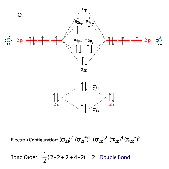
Anyway, oxygen is at first look totally not magnetic. But it seems that chemistry is not a total chaotic science at all because according to their moleluclar orbital theory it is explained that an O2 oxygen molecule has two unpaired electrons. See the next picture:
You can neglect that ‘Bond Order’ stuff.
You can think of many experimental designs in order to prove that electrons are magnetic monopoles. If my insights are correct, each and every O2 molecule must act as a magnetic monopole. That means if you apply the correct magnetic field, you can repel oxygen molecules and attract the same molecules if you flip the applied magnetic field.
If you remark that if oxygen molecules act as magnetic monopole molecules, the scientists would have found out that decades ago… But my dear reader that is not how the human mind works. If the belief is that magnetic monopoles do not exist, that causes the mind to be blind as why electrons or oxygen molecules behave as they do.
For example the electron pair is neutral when it comes to magnetic fields, how do the professional professors explain that? Well they say that the opposite magnetic fields cancel each other out. So why don’t they see they are telling crap? If the electron is a tiny magnet with a north and a south pole, isn’t that magnetically neutral to begin with? So why is the unpaired electron not magnetically neutral? At that point they begin telling stuff like ‘anti alignment’, the Pauli exclusion principle and most of all ‘quantum numbers’. It all doesn’t add up, it is crap.
That is what I had to say on this tiny detail: Likely each and every oxygen molecule with such a non binding electron pair in it will act as a magnetic monopole…