Some posts ago I showed you how you can calculate the number tau (always the logarithm of a suitable imaginary unit) using integrals for an elliptic multiplication. To be precise you can integrate the inverse of numbers along a path and that gives you the log. Just like on the real line if you start integrating in 1 and integrate 1/x you will get log(x). If you have read that post you know or remember those integrals look rather scary. And the method of using integrals is in it’s simplest on the 2D plane, in 3D real space those integrals are a lot harder to crack. And if the dimension is beyond 3 it gets worse and worse.
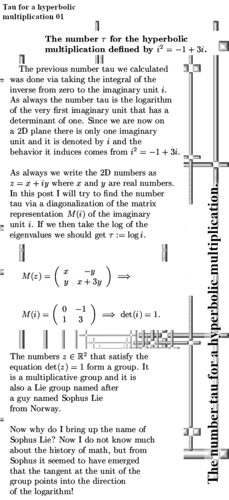
That is why many years ago I developed a method that would always work in all dimensions and that is using matrix diagonalization. If you want the log of an imaginary unit, you can diagonalize it’s matrix representation. And ok ok that too becomes a bit more cumbersome when the dimensions rise. I once calculated the number tau for seven dimensional circular numbers or if you want for 7D split complex numbers. As you might have observed for yourself: For a human such calculations are a pain in the ass because just the tiniest of mistakes lead to the wrong answer. It is just like multiplying two large numbers by hand with paper and pencil, one digit wrong and the whole thing is wrong.
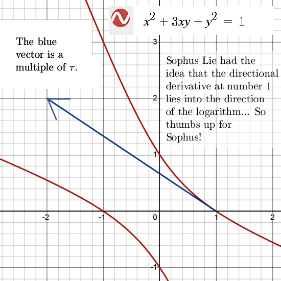
Now we are going to calculate a log in a 2D space so wouldn’t it be handy if at least beforehand we know in what direction this log will go? After all a 2D real space is also known as a plane and in a plane we have vectors and stuff.
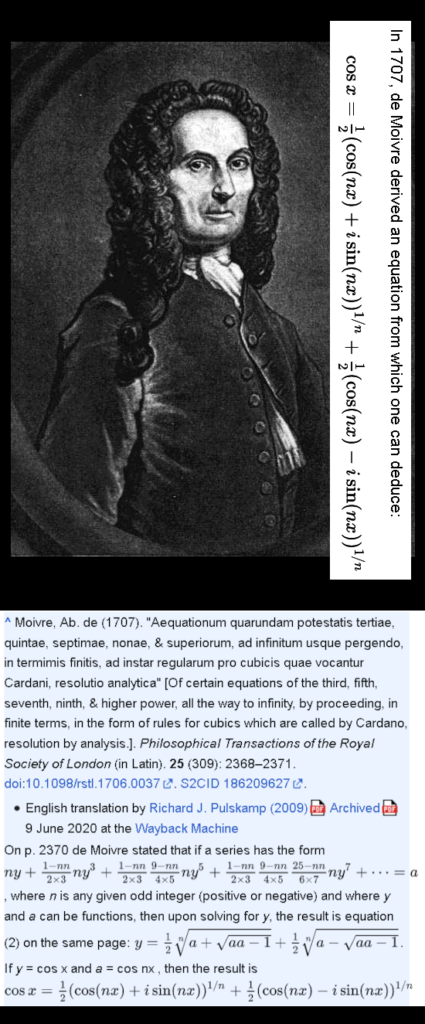
So for the very first tme after 12 years of not using it, I decided to include a very simple idea of a guy named Sophus Lie. When back in the year 2012 I decided to pick up my idea’s around higher complex numbers again of course I looked up if I could use anything from the past. And without doubt the math related to Sophus Lie was the most promising one because all other stuff was contaminated by those evil algebra people that at best use the square of an imaginary unit.
But I decided not to do it because yes indeed those Lie groups were smooth so it was related to differentiation but it also had weird stuff like the Lie bracket that I had no use for. Beside that in Lie groups and Lie algebra’s there are no Cauchy-Riemann equations. As such I just could not use it and I decided to go my own way.
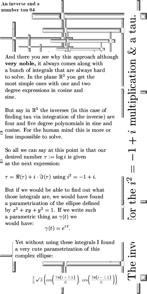
Yet in this post I use a simple idea of Sophus Lie: If you differentiate the group at 1, that vector will point into the direction of the logarithm of the imaginary unit. It’s not a very deep math result but it is very helpful. Compare it to a screwdriver, a screwdriver is not a complicated machinery but it can be very useful in case you need to screw some screws…
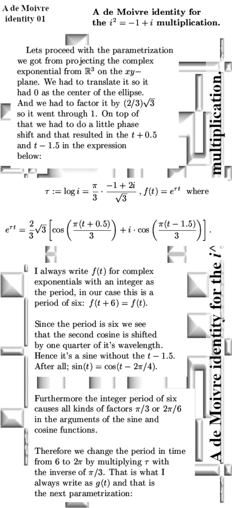
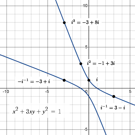
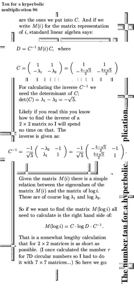
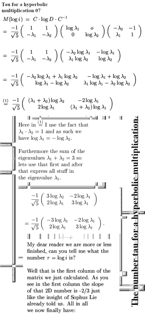
Anyway for the mulitiplication in the complex plane ruled by
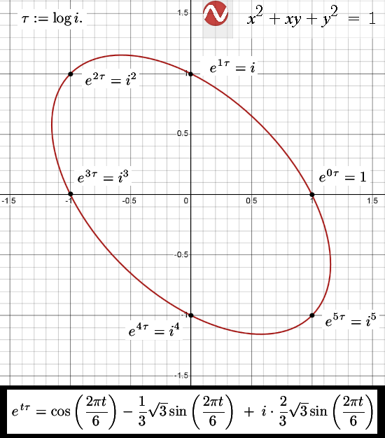
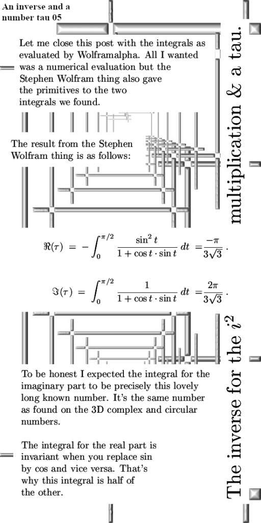
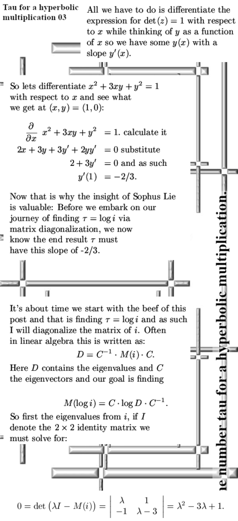
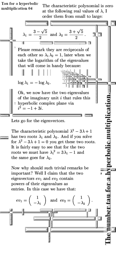
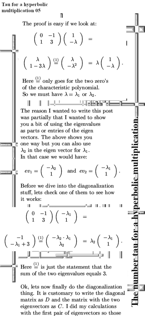
i^2 = -1 + 3i I used the method of matrix diagonalization to get the log of the imaginary unit i. So all in all it is very simple but I needed 8 pictures to pen it all down and also one extra picture know as Figure 1.
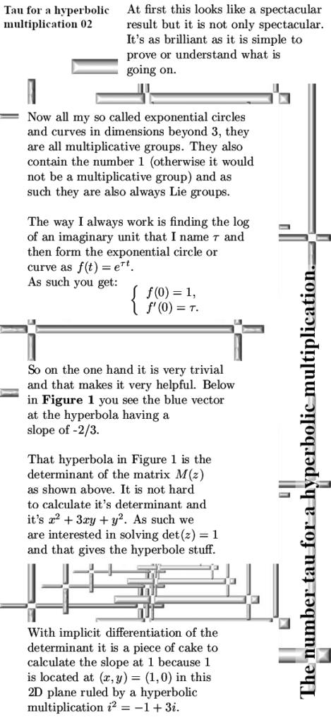
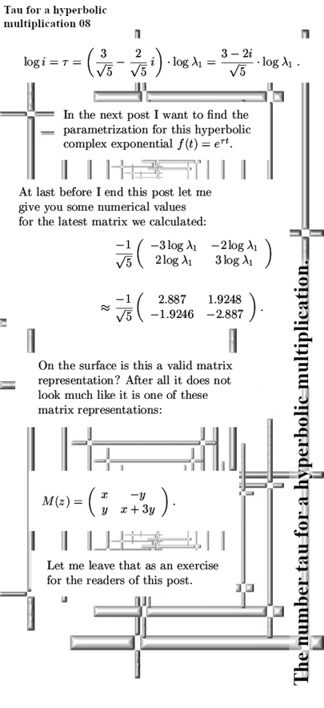
That was it for this post, we now have a number tau that is the logarithm of the imaginary unit i that rules the multiplication on this complex plane. The next post is about finding the parametrization for the hyperbole that has a determinant of 1 using this number tau.
As always thanks for your attention and see you in the next post.